AUTOMATION & CONTROL - Theory and Practice Part 4 doc

AUTOMATION&CONTROL-TheoryandPractice66


Fig. 3. Representation based on services

The reports development task allows generating some types of reports. Each of them is
focused to show an installation feature like: wired connections, devices situation, device
configuration, services…
Environment features can be used from different abstraction layers. Figure 4 shows
relationships between environment features and abstraction layer, in which are
implemented. The installation design could be used from functional, structural and
technological layers. Installation simulation can be used from functional, structural and
technological layers. Architecture modelling only supports the structural and technological
layer. It is technological because it is implemented over real devices and it is structural
because some architecture layers could be common. Making budgets is useful only from
technological layer because the budgets are for customers. Instead reports can be created
from the functional, structural and technological layers, because reports can be useful for
different applications. The customer could need a services report, a developer could need a
structural report and an installation engineer could need a wired reports.


Fig. 4. Abstraction layers supported by each feature


3.1 Resources definition
Resources of functional level are classified according to input and output resources. At
functional level resources are classified in order to determine subcategories inside input and
output resources.
Input resources are also subdivided to continuous and discrete sensors. Each family sensor
is associated to a single magnitude to measure. Continuous sensors are those which
measures continuous magnitudes like temperature, humidity, lighting, etc. Discrete sensors

are those which detect events like: gas escape, presence sensors, broken windows, etc. These
sensors indicate that an event has happened.
Output resources are subdivided into two groups: continuous and discrete actuators.
Continuous actuators are characterized because they feedback continuous sensors and
discrete do not feedback sensors. The first type is e.g. HVAC device that modifies the
magnitude measured previously by a continuous sensor. Second type is e.g. acoustic alarm
which does not invoke any event. Continuous actuators interact and modify the magnitude
measured by sensors. Continuous actuators are determined by the direct magnitude that
they modify directly and indirect magnitude list that might be modifies in any way by the
actuator, e.g. HVAC modifies directly temperature and indirectly humidity. Other aspect to
be explained is the capacity of some actuators to modify the physical structure where they
are installed, e.g. blind engine or window engine that modify the wall structure allowing or
prevent lightening and rise or fall the temperature.

3.2 Implementation
The environment has been implemented using Java and uses an information system
implemented based on XML. The XML files reflect information of resources definition that
can be used in the installation and the information about the current network. This
information is reflected from abstraction layers defined at the model. The resources reflected
in the XML files represent a subset of the features offered by market. The environment could
expand the information system adding new resources in XML files. Adding new resources is
easy because we only have to define the XML files that define the new resource and
interactions with magnitudes.
The prototyping environment presents four different areas, see figure 5. On the top of the
window, we can see the services that can be added to the network. On the left side there are
all the generic resources that can be used in the design. In the middle, there is the building
floor map. In this area services and generic resources can be added for designing the control
network. On the right side, there is hierarchical list of all the resources added in the network
classified by resource type.
The control network design starts up opening a map of the building where user can drag

and drop resources and services in order to design the network. The next action is adding
services, input and output resources into the map, after doing that, user has to connect
resources and services in order to establish relationships. Moreover, user has to configure
parameters of input and output resources and, finally, user must determine the behaviour of
each service through logical operators between input and output resources. It is not possible
link inputs and outputs resources directly because it is necessary a service that link them.
Figure 5 shows a control network designed at the environment. The control network
contains two services: HVAC and technical security. HVAC is formed by a temperature
sensor and an air-conditioning and heating. The technical security is composed by a gas
Aframeworkforsimulatinghomecontrolnetworks 67


Fig. 3. Representation based on services

The reports development task allows generating some types of reports. Each of them is
focused to show an installation feature like: wired connections, devices situation, device
configuration, services…
Environment features can be used from different abstraction layers. Figure 4 shows
relationships between environment features and abstraction layer, in which are
implemented. The installation design could be used from functional, structural and
technological layers. Installation simulation can be used from functional, structural and
technological layers. Architecture modelling only supports the structural and technological
layer. It is technological because it is implemented over real devices and it is structural
because some architecture layers could be common. Making budgets is useful only from
technological layer because the budgets are for customers. Instead reports can be created
from the functional, structural and technological layers, because reports can be useful for
different applications. The customer could need a services report, a developer could need a
structural report and an installation engineer could need a wired reports.

Fig. 4. Abstraction layers supported by each feature


3.1 Resources definition
Resources of functional level are classified according to input and output resources. At
functional level resources are classified in order to determine subcategories inside input and
output resources.
Input resources are also subdivided to continuous and discrete sensors. Each family sensor
is associated to a single magnitude to measure. Continuous sensors are those which
measures continuous magnitudes like temperature, humidity, lighting, etc. Discrete sensors
are those which detect events like: gas escape, presence sensors, broken windows, etc. These
sensors indicate that an event has happened.
Output resources are subdivided into two groups: continuous and discrete actuators.
Continuous actuators are characterized because they feedback continuous sensors and
discrete do not feedback sensors. The first type is e.g. HVAC device that modifies the
magnitude measured previously by a continuous sensor. Second type is e.g. acoustic alarm
which does not invoke any event. Continuous actuators interact and modify the magnitude
measured by sensors. Continuous actuators are determined by the direct magnitude that
they modify directly and indirect magnitude list that might be modifies in any way by the
actuator, e.g. HVAC modifies directly temperature and indirectly humidity. Other aspect to
be explained is the capacity of some actuators to modify the physical structure where they
are installed, e.g. blind engine or window engine that modify the wall structure allowing or
prevent lightening and rise or fall the temperature.

3.2 Implementation
The environment has been implemented using Java and uses an information system
implemented based on XML. The XML files reflect information of resources definition that
can be used in the installation and the information about the current network. This
information is reflected from abstraction layers defined at the model. The resources reflected
in the XML files represent a subset of the features offered by market. The environment could

expand the information system adding new resources in XML files. Adding new resources is
easy because we only have to define the XML files that define the new resource and
interactions with magnitudes.
The prototyping environment presents four different areas, see figure 5. On the top of the
window, we can see the services that can be added to the network. On the left side there are
all the generic resources that can be used in the design. In the middle, there is the building
floor map. In this area services and generic resources can be added for designing the control
network. On the right side, there is hierarchical list of all the resources added in the network
classified by resource type.
The control network design starts up opening a map of the building where user can drag
and drop resources and services in order to design the network. The next action is adding
services, input and output resources into the map, after doing that, user has to connect
resources and services in order to establish relationships. Moreover, user has to configure
parameters of input and output resources and, finally, user must determine the behaviour of
each service through logical operators between input and output resources. It is not possible
link inputs and outputs resources directly because it is necessary a service that link them.
Figure 5 shows a control network designed at the environment. The control network
contains two services: HVAC and technical security. HVAC is formed by a temperature
sensor and an air-conditioning and heating. The technical security is composed by a gas
AUTOMATION&CONTROL-TheoryandPractice68

sensor and an acoustic alarm. Although this design does not share any resource, it is
possible share resources into some services as we have show at figure 3.



Fig. 5. Environment aspect and control network design. It contains HVAC and technical
security services

Each service defines their behaviour based on some functions. These functions receive

inputs from input resources and provide outputs to output resources. Functions are
composed by logical, arithmetical or comparing operators. This specification contains
inputs, and outputs that allows interconnect them using operators. Figure 6 shows services
definition window. On the middle of the figure we can see inputs resources on the left and
output resources on the right. Operators are situated on the left side of the window and it
could be drag and drop into the previous area in order to link inputs and outputs. Operators
should be configured in order to define the behaviour of the service. This figure contains the
HVAC service behaviour. Refrigerator will be turned on when temperature rises above 25
Celsius degrees and it will be turned off when temperature falls under 25 Celsius degrees.
Heating will be turn on when temperature reaches 15 Celsius degrees and it will be turn off
when temperature rises above 15 Celsius degrees. According to this parameters temperature
will be between 15 and 25 Celsius degrees.



Fig. 6. HVAC performance is defined by logical operators

4. Simulation

The environment is designed to perform simulations from different abstraction levels.
Environment simulates from functional layer Eq. (1), Eq. (2), structural layer Eq. (3), Eq. (4)
and Eq. (5) and technological layer Eq. (6). The functional simulation is responsible for
simulating the behaviour of generic control network. With this validation we can be sure
that generic device configuration and connections are correct. The structural simulation
includes the functional, but adds new features, like the real position of the resources and
installation regulation. The technological simulation determines the real behaviour that the
implemented control network is going to provide.
Functional layer simulating it is explained. This simulation is determined by two
parameters: simulation time and frequency. The first one represents the interval we want to
simulate. The second is the number of values from each resource that we will take in a time

unit.
Simulation task needs a flag for continuous and discrete sensors. This action is carried out
by event generators. We have designed two event generator types, discrete event generator
and continuous event generator. The first type gives up data for discrete sensors, and is
based on probability percentage, that is defined for each discrete sensor in the network. The
second type represents input data for continuous sensors and is based on medium value and
variation value throughout simulation time. Obtaining a sinusoidal wave which represents
continuous magnitudes like temperature, humidity, etc
The results are represented in two views. The first one shows building map, control network
and resources values are drawn under their own resource. Resources values are changing at
a given frequency in order to view the evolution of the control network in simulation time.
This view is showed in figure 7.

Aframeworkforsimulatinghomecontrolnetworks 69

sensor and an acoustic alarm. Although this design does not share any resource, it is
possible share resources into some services as we have show at figure 3.



Fig. 5. Environment aspect and control network design. It contains HVAC and technical
security services

Each service defines their behaviour based on some functions. These functions receive
inputs from input resources and provide outputs to output resources. Functions are
composed by logical, arithmetical or comparing operators. This specification contains
inputs, and outputs that allows interconnect them using operators. Figure 6 shows services
definition window. On the middle of the figure we can see inputs resources on the left and
output resources on the right. Operators are situated on the left side of the window and it
could be drag and drop into the previous area in order to link inputs and outputs. Operators

should be configured in order to define the behaviour of the service. This figure contains the
HVAC service behaviour. Refrigerator will be turned on when temperature rises above 25
Celsius degrees and it will be turned off when temperature falls under 25 Celsius degrees.
Heating will be turn on when temperature reaches 15 Celsius degrees and it will be turn off
when temperature rises above 15 Celsius degrees. According to this parameters temperature
will be between 15 and 25 Celsius degrees.



Fig. 6. HVAC performance is defined by logical operators

4. Simulation

The environment is designed to perform simulations from different abstraction levels.
Environment simulates from functional layer Eq. (1), Eq. (2), structural layer Eq. (3), Eq. (4)
and Eq. (5) and technological layer Eq. (6). The functional simulation is responsible for
simulating the behaviour of generic control network. With this validation we can be sure
that generic device configuration and connections are correct. The structural simulation
includes the functional, but adds new features, like the real position of the resources and
installation regulation. The technological simulation determines the real behaviour that the
implemented control network is going to provide.
Functional layer simulating it is explained. This simulation is determined by two
parameters: simulation time and frequency. The first one represents the interval we want to
simulate. The second is the number of values from each resource that we will take in a time
unit.
Simulation task needs a flag for continuous and discrete sensors. This action is carried out
by event generators. We have designed two event generator types, discrete event generator
and continuous event generator. The first type gives up data for discrete sensors, and is
based on probability percentage, that is defined for each discrete sensor in the network. The
second type represents input data for continuous sensors and is based on medium value and

variation value throughout simulation time. Obtaining a sinusoidal wave which represents
continuous magnitudes like temperature, humidity, etc
The results are represented in two views. The first one shows building map, control network
and resources values are drawn under their own resource. Resources values are changing at
a given frequency in order to view the evolution of the control network in simulation time.
This view is showed in figure 7.

AUTOMATION&CONTROL-TheoryandPractice70


Fig. 7. Simulation results view showing values at the frequency defined at the top of the
window

The second view represents a graph. A graph is showed for each resource in the previous
view. The graph represents the resource behaviour in simulation time. There are three types
of graphs.
The first graph type shows services. This graph shows all signals of the resources linked in
the service, representing all the information in one graph, although sometimes data range
are different so we have to view graphs individually at each resource. Thinking in our
HVAC service example, the graph shows temperature sensor, air-conditioning and heating
values. The second graph type represents sensors and shows event generators values and
values given by the sensor. In HVAC example, the temperature sensor graph shows external
temperature and the temperature sensor measured, which might have a little error. The
third graph is reserved for actuators, and shows actuator values drawn as a single signal
representing the actuator performance. In HVAC example, the air-conditioning and heating
will be show in two graphs, each one shows a signal indicating when the air-conditioning is
on or off. Figure 8 shows three graphs, temperature sensor at left, air-conditioning at right
on top and heating at right on bottom. Temperature sensor graph shows the external
temperature in blue, which is generated as a variation event, and sensor temperature in red.
The red signal has peaks because the sensor has been defined with measure error. Moreover

the red signal is ever between 25 and 15 Celsius degrees because the air-conditioning starts

when temperature rises and the heating starts when temperature falls. Air-conditioning and
heating graph shows when they start to work.


Fig. 8. Simulation results graph of temperature sensor, air-conditioning and heating

4.1 Implementation
Simulation is realized by an external module. It is implemented in external way to leave us
introduce future changes in the simulation module esaily, without impact for the
environment. It has been developed in Matlab / Simulink because allows high precision and
efficiency.
The communication between the simulation module and environment has been done
through a Java library called jMatLink (Müller & Waller, 1999). It is responsible for sending
commands to Matlab. This action requires knowing Matlab commands perfectly. We have
developed a library called jSCA. It is responsible for encapsulating Matlab commands to
facilitate the communication. The features of jSCA are implemented as method which
allows: create instances of Matlab; create, configure, and remove blocks in Simulink;
configure parameters simulation, and obtain the results of the simulation. This library is a
level above jMatLink. The environment make calls to jSCA library and this library calls to
jMatlink library.
The architecture that achieves the communication between Java application and Simulink is
showed at figure 9. The first three layers are inside the environment, but the latter two are
external environment. The first layer is the own prototyping environment. The second one is
the jSCA library. The third one is jMatlink library. The fourth is Matlab engine. It is a
daemon that is listening commands thrown by jMatlink. We use Matlab Engine as
middleware between jMatLink and Simulink. So we launch Simulink and throws commands
through Matlab Engine.
The interaction between the user and the architecture layers defined previously is showed

by a sequence diagram. This diagram shows temporal sequence of main calls. Figure 10
shows the sequence diagram, which corresponds to a specification language: Unified
Modelling Language (UML). Temporal sequences of calls begin when user designs the
Aframeworkforsimulatinghomecontrolnetworks 71


Fig. 7. Simulation results view showing values at the frequency defined at the top of the
window

The second view represents a graph. A graph is showed for each resource in the previous
view. The graph represents the resource behaviour in simulation time. There are three types
of graphs.
The first graph type shows services. This graph shows all signals of the resources linked in
the service, representing all the information in one graph, although sometimes data range
are different so we have to view graphs individually at each resource. Thinking in our
HVAC service example, the graph shows temperature sensor, air-conditioning and heating
values. The second graph type represents sensors and shows event generators values and
values given by the sensor. In HVAC example, the temperature sensor graph shows external
temperature and the temperature sensor measured, which might have a little error. The
third graph is reserved for actuators, and shows actuator values drawn as a single signal
representing the actuator performance. In HVAC example, the air-conditioning and heating
will be show in two graphs, each one shows a signal indicating when the air-conditioning is
on or off. Figure 8 shows three graphs, temperature sensor at left, air-conditioning at right
on top and heating at right on bottom. Temperature sensor graph shows the external
temperature in blue, which is generated as a variation event, and sensor temperature in red.
The red signal has peaks because the sensor has been defined with measure error. Moreover
the red signal is ever between 25 and 15 Celsius degrees because the air-conditioning starts

when temperature rises and the heating starts when temperature falls. Air-conditioning and
heating graph shows when they start to work.

Fig. 8. Simulation results graph of temperature sensor, air-conditioning and heating

4.1 Implementation
Simulation is realized by an external module. It is implemented in external way to leave us
introduce future changes in the simulation module esaily, without impact for the
environment. It has been developed in Matlab / Simulink because allows high precision and
efficiency.
The communication between the simulation module and environment has been done
through a Java library called jMatLink (Müller & Waller, 1999). It is responsible for sending
commands to Matlab. This action requires knowing Matlab commands perfectly. We have
developed a library called jSCA. It is responsible for encapsulating Matlab commands to
facilitate the communication. The features of jSCA are implemented as method which
allows: create instances of Matlab; create, configure, and remove blocks in Simulink;
configure parameters simulation, and obtain the results of the simulation. This library is a
level above jMatLink. The environment make calls to jSCA library and this library calls to
jMatlink library.
The architecture that achieves the communication between Java application and Simulink is
showed at figure 9. The first three layers are inside the environment, but the latter two are
external environment. The first layer is the own prototyping environment. The second one is
the jSCA library. The third one is jMatlink library. The fourth is Matlab engine. It is a
daemon that is listening commands thrown by jMatlink. We use Matlab Engine as
middleware between jMatLink and Simulink. So we launch Simulink and throws commands
through Matlab Engine.
The interaction between the user and the architecture layers defined previously is showed
by a sequence diagram. This diagram shows temporal sequence of main calls. Figure 10
shows the sequence diagram, which corresponds to a specification language: Unified
Modelling Language (UML). Temporal sequences of calls begin when user designs the
AUTOMATION&CONTROL-TheoryandPractice72

co
n
jM
cr
e
m
d
fi
n
tr
a

Fi
g

F
u
m
o
en
v
in
bl
o
co
n
an

Fi

g
ar
c

n
trol network. T
h
M
atlink la
y
er to c
r
e
ate the mdl file
.
d
l has been crea
t
n
ish, simulation
v
a
s
g
u visualizes it.
g
. 9. Architecture

u
nctional simulat

i
o
del is equivale
n
v
ironment. Each

Simuli
n
k. The S
i
o
cks, output-blo
c
n
tinuous. The d
i
alo
g
ical devices.

g
. 10. Sequenc
e
c
hitecture
h
e next action i
s
r

eateMDL file. T
h
.
Finall
y
, Matlab

t
ed Matlab en
g
i
n
v
alues are retur
n


that achieves co
m
i
o
n
requires a p
a
n
t to resources X
M

resource define
d

i
mulink model c
o
c
ks and input-ou
t
i
screte blocks ar

e
dia
g
ram that
s
to simulate it.
I
h
is la
y
er starts
M

en
g
ine calls Si
m
n
e calls Simulin
k
n

ed la
y
er after
l
m
munication am
a
rallel model fro
m
M
L files defined

d
in the environ
m
o
nsists on a bloc
k
t
put blocks. The
r
e dedicated to
d
shows the int
e
I
f user starts sim
M
atlab server an
d

m
ulink and it cre
a
k
for start simul
a
l
a
y
er until tras
gu

o
n
g
Java applica
t
m
the functional

in the informati
m
ent is correspon
d
k
set formed b
y

i
r

e are also two b
l
d
i
g
ital devices,
a
e
raction amon
g

ulation tras
g
u
w
d
calls Matlab en
g
a
tes the mdl file
a
tion. When sim
u
u
received it an
d
t
ion and Simulin
k
la

y
er i
n
Simulin
k
on system used
d
ed b
y
another
d
i
nput blocks, co
n
l
ock t
y
pes: discr
e
a
nd continuous
a

user and sim
u
w
ill call
g
ine to
. Once

u
lation
d
then
k

k
. This
by the
d
efined
n
troller
e
te and
a
re for
u
lation

The simulation starts creating an equivalent control network in Simulink dynamically. The
Simulink control network is saved into mdl file. To create the mdl file, we add the
corresponding network blocks. Parameters of each block are configured and connections
among blocks are created. The next step is to add probability or variation events for each
sensor. Through these events the input resources are activated and we can see how the
network reacts. The last step is to feedback the signal from actuators to sensors, adding
actuators outputs and original event, obtaining real value.
An example of this Simulink network is showed on figure 11. It shows, at section I, events
generators and adding block that represent feedback. Each input resource has a
correspondent event generator: discrete or continuous. Section II has input resources.

Section III shows services which join input and output resources. Services definitions are
made recursively by others mdl files. These mdl files are equivalent to the services defined
at environment. At section IV we have output resources. Finally, section V shows feedback
generated by actuators, which modify measured magnitudes. The feedback is adjusted in
function of how we have configured the actuator at the environment. Each section shows a
white box connected to each resource. These boxes store a value list obtained from
simulation. This list contains discrete values taken at given frequency.


Fig. 11. Simulink control network generated dynamically from a previous design made at
the environment

When the mdl file is created, Simulink executes the simulation and the environment reads
all variable lists from Simulink and represents them at the given frequency in the view
defined previously at environment. This way, the simulation is not interactive, when the
Aframeworkforsimulatinghomecontrolnetworks 73

co
n
jM
cr
e
m
d
fi
n
tr
a

Fi

g

F
u
m
o
en
v
in
bl
o
co
n
an

Fi
g
ar
c

n
trol network. T
h
M
atlink la
y
er to c
r
e
ate the mdl file

.
d
l has been crea
t
n
ish, simulation
v
a
s
g
u visualizes it.
g
. 9. Architecture

u
nctional simulat
i
o
del is equivale
n
v
ironment. Each

Simuli
n
k. The S
i
o
cks, output-blo
c

n
tinuous. The d
i
alo
g
ical devices.

g
. 10. Sequenc
e
c
hitecture
h
e next action i
s
r
eateMDL file. T
h
.
Finall
y
, Matlab

t
ed Matlab en
g
i
n
v
alues are retur

n


that achieves co
m
i
o
n
requires a p
a
n
t to resources X
M

resource define
d
i
mulink model c
o
c
ks and input-ou
t
i
screte blocks ar

e
dia
g
ram that
s

to simulate it.
I
h
is la
y
er starts
M

en
g
ine calls Si
m
n
e calls Simulin
k
n
ed la
y
er after
l
m
munication am
a
rallel model fro
m
M
L files defined

d
in the environ

m
o
nsists on a bloc
k
t
put blocks. The
r
e dedicated to
d
shows the int
e
I
f user starts sim
M
atlab server an
d
m
ulink and it cre
a
k
for start simul
a
l
a
y
er until tras
gu

o
n

g
Java applica
t
m
the functional

in the informati
m
ent is correspon
d
k
set formed b
y

i
r
e are also two b
l
d
i
g
ital devices,
a
e
raction amon
g

ulation tras
g
u

w
d
calls Matlab en
g
a
tes the mdl file
a
tion. When sim
u
u
received it an
d
t
ion and Simulin
k
la
y
er i
n
Simulin
k
on s
y
stem used
d
ed b
y
another
d
i

nput blocks, co
n
l
ock t
y
pes: discr
e
a
nd continuous
a

user and sim
u
w
ill call
g
ine to
. Once
u
lation
d
then
k

k
. This
b
y
the
d

efined
n
troller
e
te and
a
re for
u
lation

The simulation starts creating an equivalent control network in Simulink dynamically. The
Simulink control network is saved into mdl file. To create the mdl file, we add the
corresponding network blocks. Parameters of each block are configured and connections
among blocks are created. The next step is to add probability or variation events for each
sensor. Through these events the input resources are activated and we can see how the
network reacts. The last step is to feedback the signal from actuators to sensors, adding
actuators outputs and original event, obtaining real value.
An example of this Simulink network is showed on figure 11. It shows, at section I, events
generators and adding block that represent feedback. Each input resource has a
correspondent event generator: discrete or continuous. Section II has input resources.
Section III shows services which join input and output resources. Services definitions are
made recursively by others mdl files. These mdl files are equivalent to the services defined
at environment. At section IV we have output resources. Finally, section V shows feedback
generated by actuators, which modify measured magnitudes. The feedback is adjusted in
function of how we have configured the actuator at the environment. Each section shows a
white box connected to each resource. These boxes store a value list obtained from
simulation. This list contains discrete values taken at given frequency.


Fig. 11. Simulink control network generated dynamically from a previous design made at

the environment

When the mdl file is created, Simulink executes the simulation and the environment reads
all variable lists from Simulink and represents them at the given frequency in the view
defined previously at environment. This way, the simulation is not interactive, when the
AUTOMATION&CONTROL-TheoryandPractice74

simulation process is launched, the user has to wait until Simulink returns the results of the
simulation.


Fig. 12. HVAC service created in Simulink from the design made at environment

Figure 12 shows the mdl file that defines a HVAC service designed previously at
environment on figure 6. At left side, input resources connection can be viewed as white
circles, in this case temperature sensor. In the middle, we there are conversion data type
blocks for avoiding Simulink data type errors and comparison operators that defines when
the actuators will start to work. Actuators are drawn as white circle on the right.

5. Conclusions

This chapter presents a prototyping environment for the design and simulation of control
networks in some areas: digital home, intelligent building. The objective is to facilitate the
tasks of designing and validating control networks. We propose a top-down methodology,
where technology implementation choice is left to the last phase of designing process. The
environment kernel is the control network model around different abstraction layers:
functional, structural and technological.
The model is the basis on which the environment gets applications by particularization:
network design, simulation, specifying architectures, developing reports, budgets, and so
on.

Simulation is presented as an intermediate phase in methodology of design control network.
It reduces costs and helps us to design effective and efficient control networks.
Future work is aimed to provide competitive solutions in the design of control networks.
The nature of the problem requires addressing increasingly scientific and technological
aspects of the problem. Therefore, in short term, we deepening in aspects of generalization
of the results: new models for structural and technological layers, an interactive simulation
module and simulation of technological layer… In long term we are going to generalize to
others context like industrial buildings, office buildings…

6. References

Balci, O., 1998. Verification, validation, and testing. In The Handbook of Simulation. John
Wiley & Sons.
Bravo, C., Redondo, M.A., Bravo, J., and Ortega, M., 2000. DOMOSIMCOL: A Simulation
Collaborative Environment for the Learning of Domotic Design. ACM SIGCSE
Bulletin, Vol. 32, No. 2, 65-67.
Bravo, C., Redondo, M., Ortega, M , and Verdejo, M.F., 2006. Collaborative environments
for the learning of design: a model and a case study in Domotics. Computers &
Education, Vol. 46, No. 2, 152-173.
Breslau, L. Estrin, D. Fall, K. Floyd, S. Heidemann, J. Helmy, A. Huang, P. McCanne, S.
Varadhan, K. Ya Xu Haobo Yu. 2000. Advances in network simulation. Computer,
Vol. 33, Issue: 5, pp: 59-67. ISSN: 0018-9162.
Conte, G. Scaradozzi, D. Perdon, A. Cesaretti, M. Morganti, G. 2007. A simulation
environment for the analysis of home automation systems. Control & Automation,
2007. MED '07. Mediterranean Conference on, pp: 1-8, ISBN: 978-1-4244-1282-2
Denning, P. J., Comer, D. E., Gries, D., Michael Mulder, C., Tucker, A., Turner, A. J., Young,
P. R., 1989. Computing as a discipline. Communications of the ACM, Vol.32 No.1,
9-23
Fuster, A. and Azorín, J., 2005. Arquitectura de Sistemas para el hogar digital. Hogar digital.
El camino de la domótica a los ambientes inteligentesI Encuentro Interdisciplinar

de Domótica 2005, pp 35-44
Fuster, A., de Miguel, G. and Azorín, J., 2005. Tecnología Middleware para pasarelas
residenciales. Hogar digital. El camino de la domótica a los ambientes inteligentes.I
Encuentro Interdisciplinar de Domótica 2005, 87-102.
González, V. M., Mateos, F., López, A.M., Enguita, J.M., García M.and Olaiz, R., 2001. Visir,
a simulation software for domotics installations to improve laboratory training,
Frontiers in Education Conference, 31st Annual Vol. 3, F4C-6-11.
Haenselmann, T., King, T., Busse, B., Effelsberg, W. and Markus Fuchs, 2007. Scriptable
Sensor Network Based Home-Automation. Emerging Directions in Embedded and
Ubiquitous Computing, 579-591.
Jung, J., Park, K. and Cha J., 2005. Implementation of a Network-Based Distributed System
Using the CAN Protocol. Knowledge-Based Intelligent Information and
Engineering Systems. Vol. 3681.
Kawamura, R. and Maeomichi, 2004. Standardization Activity of OSGi (Open Services
Gateway Initiative), NTT Technical Review, Vol. 2, No. 1, 94-97.
Mellor, S., Scott K., Uhl, A. and Weise, D., 2004. MDA Distilled, Principles of Model Driven
Architecture, Addison-Wesley Professional.
Min, W., Hong, Z., Guo-ping, L. and Jin-hua, S., 2007. Networked control and supervision
system based on LonWorks fieldbus and Intranet/Internet. Journal of Central
South University of Technology, Vol. 14, No.2, 260-265.
Moya, F. and López, J.C., 2002 .SENDA: An Alternative to OSGi for Large Scale Domotics.
Networks, pp. 165-176.
Müller, S. and Waller, H., 1999. Efficient Integration of Real-Time Hardware and Web Based
Services Into MATLAB. 11
th
European Simulation Symposium and Exhibition, 26-
28.
Aframeworkforsimulatinghomecontrolnetworks 75

simulation process is launched, the user has to wait until Simulink returns the results of the

simulation.


Fig. 12. HVAC service created in Simulink from the design made at environment

Figure 12 shows the mdl file that defines a HVAC service designed previously at
environment on figure 6. At left side, input resources connection can be viewed as white
circles, in this case temperature sensor. In the middle, we there are conversion data type
blocks for avoiding Simulink data type errors and comparison operators that defines when
the actuators will start to work. Actuators are drawn as white circle on the right.

5. Conclusions

This chapter presents a prototyping environment for the design and simulation of control
networks in some areas: digital home, intelligent building. The objective is to facilitate the
tasks of designing and validating control networks. We propose a top-down methodology,
where technology implementation choice is left to the last phase of designing process. The
environment kernel is the control network model around different abstraction layers:
functional, structural and technological.
The model is the basis on which the environment gets applications by particularization:
network design, simulation, specifying architectures, developing reports, budgets, and so
on.
Simulation is presented as an intermediate phase in methodology of design control network.
It reduces costs and helps us to design effective and efficient control networks.
Future work is aimed to provide competitive solutions in the design of control networks.
The nature of the problem requires addressing increasingly scientific and technological
aspects of the problem. Therefore, in short term, we deepening in aspects of generalization
of the results: new models for structural and technological layers, an interactive simulation
module and simulation of technological layer… In long term we are going to generalize to
others context like industrial buildings, office buildings…

6. References

Balci, O., 1998. Verification, validation, and testing. In The Handbook of Simulation. John
Wiley & Sons.
Bravo, C., Redondo, M.A., Bravo, J., and Ortega, M., 2000. DOMOSIMCOL: A Simulation
Collaborative Environment for the Learning of Domotic Design. ACM SIGCSE
Bulletin, Vol. 32, No. 2, 65-67.
Bravo, C., Redondo, M., Ortega, M , and Verdejo, M.F., 2006. Collaborative environments
for the learning of design: a model and a case study in Domotics. Computers &
Education, Vol. 46, No. 2, 152-173.
Breslau, L. Estrin, D. Fall, K. Floyd, S. Heidemann, J. Helmy, A. Huang, P. McCanne, S.
Varadhan, K. Ya Xu Haobo Yu. 2000. Advances in network simulation. Computer,
Vol. 33, Issue: 5, pp: 59-67. ISSN: 0018-9162.
Conte, G. Scaradozzi, D. Perdon, A. Cesaretti, M. Morganti, G. 2007. A simulation
environment for the analysis of home automation systems. Control & Automation,
2007. MED '07. Mediterranean Conference on, pp: 1-8, ISBN: 978-1-4244-1282-2
Denning, P. J., Comer, D. E., Gries, D., Michael Mulder, C., Tucker, A., Turner, A. J., Young,
P. R., 1989. Computing as a discipline. Communications of the ACM, Vol.32 No.1,
9-23
Fuster, A. and Azorín, J., 2005. Arquitectura de Sistemas para el hogar digital. Hogar digital.
El camino de la domótica a los ambientes inteligentesI Encuentro Interdisciplinar
de Domótica 2005, pp 35-44
Fuster, A., de Miguel, G. and Azorín, J., 2005. Tecnología Middleware para pasarelas
residenciales. Hogar digital. El camino de la domótica a los ambientes inteligentes.I
Encuentro Interdisciplinar de Domótica 2005, 87-102.
González, V. M., Mateos, F., López, A.M., Enguita, J.M., García M.and Olaiz, R., 2001. Visir,
a simulation software for domotics installations to improve laboratory training,
Frontiers in Education Conference, 31st Annual Vol. 3, F4C-6-11.
Haenselmann, T., King, T., Busse, B., Effelsberg, W. and Markus Fuchs, 2007. Scriptable

Sensor Network Based Home-Automation. Emerging Directions in Embedded and
Ubiquitous Computing, 579-591.
Jung, J., Park, K. and Cha J., 2005. Implementation of a Network-Based Distributed System
Using the CAN Protocol. Knowledge-Based Intelligent Information and
Engineering Systems. Vol. 3681.
Kawamura, R. and Maeomichi, 2004. Standardization Activity of OSGi (Open Services
Gateway Initiative), NTT Technical Review, Vol. 2, No. 1, 94-97.
Mellor, S., Scott K., Uhl, A. and Weise, D., 2004. MDA Distilled, Principles of Model Driven
Architecture, Addison-Wesley Professional.
Min, W., Hong, Z., Guo-ping, L. and Jin-hua, S., 2007. Networked control and supervision
system based on LonWorks fieldbus and Intranet/Internet. Journal of Central
South University of Technology, Vol. 14, No.2, 260-265.
Moya, F. and López, J.C., 2002 .SENDA: An Alternative to OSGi for Large Scale Domotics.
Networks, pp. 165-176.
Müller, S. and Waller, H., 1999. Efficient Integration of Real-Time Hardware and Web Based
Services Into MATLAB. 11
th
European Simulation Symposium and Exhibition, 26-
28.
AUTOMATION&CONTROL-TheoryandPractice76

Muñoz, J., Fons, J., Pelechano, V. and Pastor, O., 2003. Hacia el Modelado Conceptual de
Sistemas Domóticos, Actas de las VIII Jornadas de Ingeniería del Software y Bases
de Datos. Universidad de Alicante, 369-378
Newcomer, E. and Lomow, G., 2005. Understanding SOA with Web Services. Addison
Wesley.
Norton S. and Suppe F., 2001. Why atmospheric modeling is good science. MIT Press. p. 88-
133.
Pan, M. and Tseng, Y. 2007. ZigBee and Their Applications. Sensor Networks and
Configuration. Ed. Springer Berlin Heidelberg, pp:349-368 ISBN:978-3-540-37364-3

Rhee, S., Yang, S., Park, S., Chun, J.and Park, J., 2004. UPnP Home Networking-Based
IEEE1394 Digital Home Appliances Control. Advanced Web Technologies and
Applications, Vol. 3007, 457-466.
Sommerville, I. 2004. Software Engineering, 7th ed. Boston: Addison-Wesley.
Sun Microsystems Inc, 1999. JINI Architectural Overview, Technical White Paper, 1999
Valdivieso, R.J., Sánchez, J.G., Azorín, J. and Fuster, A., 2007. Entorno para el desarrollo y
simulación de arquitecturas de redes de control en el hogar. II Internacional
Simposium Ubiquitous Computing and Ambient Intelligence.

ComparisonofDefuzzicationMethods:
AutomaticControlofTemperatureandFlowinHeatExchanger 77
Comparison of Defuzzication Methods: Automatic Control of
TemperatureandFlowinHeatExchanger
AlvaroJ.ReyAmaya,OmarLengerke,CarlosA.Cosenza,MaxSuellDutraandMagda
J.M.Tavera
X

Comparison of Defuzzification Methods:
Automatic Control of Temperature
and Flow inHeat Exchanger

Alvaro J. Rey Amaya
†
, Omar Lengerke
†
, Carlos A. Cosenza

,
Max Suell Dutra


and Magda J.M. Tavera


†
Autonomous University of Bucaramanga – UNAB,
Calle 48 # 39 -234, Bucaramanga - Colombia

Federal University of Rio de Janeiro – COPPE-UFRJ
Postal Box 68.503 – CEP 21.945-970 – Rio de Janeiro, RJ, Brazil

1. Introduction

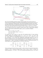
The purpose of this work is to analyze the behavior of traditional and fuzzy control,
applying in flow and temperature control to load current of a heat exchanger, and the
analysis of different methods of defuzzification, utilized just as itself this carrying out the
fuzzy control. Acting on the fuzzy controller structure, some changes of form are carried out
such that this tune in to be able to obtain optimal response. Proceeds on the traditional
controller and comparisons techniques on these two types of controls are established. Inside
the changes that are carried out on the fuzzy controller this form of information
defuzzification, that is to say the methods are exchanged defuzzification in order then to
realize comparisons on the behavior of each one of methods.
In many sectors of the industry where include thermal processes, is important the presence
of heat exchangers (Shah & Sekulic, 2003, Kuppan, 2000). Said processes are components of
everyday life of an engineer that has as action field the control systems, therefore is
considered interesting to realize a control to this type of systems. This work studies two
significant aspects: A comparison between traditional and fuzzy control, and an analysis
between several defuzzification methods utilized in the fuzzy logic (Kovacic & Bogdan,
2006, Harris, 2006), development an analysis on each one of methods taking into
consideration, contribute that other authors have done and leaving always in allow, that the

alone results obtained will be applicable at the time of execute control on an heat exchanger
(Xia et al., 1991, Fischer et al., 1998, Alotaibi et al., 2004,). The test system this composed for
two heat exchangers, one of concentric pipes and other of hull and pipes, to which
implemented them a temperature and flow automatic control to the load current of heating
(Fig. 1).

6
AUTOMATION&CONTROL-TheoryandPractice78


Fig. 1. Thermal pilot plant scheme

The control is realized through two proportional valves, one on input of the water,
responsible for keep the value of order of the water and other installed in the line of input of
the vapor (source of heat), responsible of keep the quantity necessary of vapor to obtain the
target temperature. Physical experimentation typically attaches the notions of uncertainty to
measurements of any physical property state (Youden, 1998). The measurement of the flow
is realized by a sensor of rotary palette and the measurement of the temperature by
thermocouples (Eckert & Goldstein, 1970, McMillan & Considine, 1999, Morris, 2001). The
signals supplied by sensors are acquired by National Instruments
®
FieldPoint module
(Kehtarnavaz & Kim, 2005, Archila et al., 2006, Blume, 2007) that takes charge and send
signal to the control valves, after to be processed the data by controller.

2. Fuzzy and Classic Control Software

The control software designed uses two sections, the fuzzy and PID
(Proportional/Integral/Derivative) control program. These controllers are created on
environment Labwindows/CVI by National Instruments Company

®
, which permits to
realize the pertinent operations with the data captured through FieldPoint modules, utilized
in systems control. The fuzzy control interface, is the responsible for receiving data of
sensors, so much of temperature for the temperature control case, as of the flow sensor for
control of the same one, to process, and according to an order established, to determine an
response sent to the actuators. Basically, this program is responsible of to schematize the
fuzzy sets, according to established by the user, defuzzification of the inputs, to realize the
inference of these inputs in rules, to realize aggregation in the outputs sets, and to execute
the defuzzification process, to determine the response that assist to the system to obtain the
established state. The PID control classic interface is similar of fuzzy control interface, but
the difference is in entrusted of to execute the three control actions, proportional, derivative
and integral to determine the responses that assist to the system to obtain its target state.

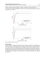
The PID control system general is represented in figure 2, where R(s), is the signal target or
set point, U(s), is the output of the PID controller that goes in the direction of the plant G(s),
and Y(s), is the value in use of the variable to control, which reduces to the reference and the
error is determined (controller input).


Fig. 2. General PID Control System

The purpose of temperature control is to achieve that water that the heat exchanger
overtakes the value of target temperature and to keep it in the value even with external
disruptions. On operate control valve is supplies the quantity of vapor that heats water. The
input to system control is the temperature error, obtained since the thermocouple placed on
the exit of the exchanger, and the exit control the quantity of necessary current to open or to
close the proportional valve (Plant). This control is realized through a PID controller.
The flow control has as purpose to obtain that water mass flow that enters to heat
exchanger, achieve the target value, and can to keep it during its operation, and even with

disruptions. This means that should operate on the valve of control, who is the one that
restrain the water quantity that enters to the system. The system input will be the error
obtained through the flow sensor installed in the input of the system, and the PID controller
will control the quantity of necessary current to manipulate the proportional valve. Both
processes begin, calculating the difference between the measured temperature and the
temperature desired or flow measured and flow desired. In this form, identify the error.
The values of control parameters are taken, and the output is calculated that goes in the
direction of the plant. This output obtains values since 0 to 20 mA, they will represent
aperture angles of proportional valve.

3. Fuzzy Control System

The inputs to control system are temperature error and gradient, obtained since the sensor
placed on the way out of exchanger, and the exit control the quantity current necessary to
open the proportional valve. The rules and membership function system are obtained in
table 1 and figure 3, respectively.

Error
Δ Error
Negative Zero Positive
Negative Open Open Not operation
Zero Open Not operation Close
Positive Not operation Close Close
Table 1. Temperature control rules assembly
ComparisonofDefuzzicationMethods:
AutomaticControlofTemperatureandFlowinHeatExchanger 79


Fig. 1. Thermal pilot plant scheme

The control is realized through two proportional valves, one on input of the water,
responsible for keep the value of order of the water and other installed in the line of input of
the vapor (source of heat), responsible of keep the quantity necessary of vapor to obtain the
target temperature. Physical experimentation typically attaches the notions of uncertainty to
measurements of any physical property state (Youden, 1998). The measurement of the flow
is realized by a sensor of rotary palette and the measurement of the temperature by
thermocouples (Eckert & Goldstein, 1970, McMillan & Considine, 1999, Morris, 2001). The
signals supplied by sensors are acquired by National Instruments
®
FieldPoint module
(Kehtarnavaz & Kim, 2005, Archila et al., 2006, Blume, 2007) that takes charge and send
signal to the control valves, after to be processed the data by controller.

2. Fuzzy and Classic Control Software

The control software designed uses two sections, the fuzzy and PID
(Proportional/Integral/Derivative) control program. These controllers are created on
environment Labwindows/CVI by National Instruments Company
®
, which permits to
realize the pertinent operations with the data captured through FieldPoint modules, utilized
in systems control. The fuzzy control interface, is the responsible for receiving data of
sensors, so much of temperature for the temperature control case, as of the flow sensor for
control of the same one, to process, and according to an order established, to determine an
response sent to the actuators. Basically, this program is responsible of to schematize the
fuzzy sets, according to established by the user, defuzzification of the inputs, to realize the
inference of these inputs in rules, to realize aggregation in the outputs sets, and to execute
the defuzzification process, to determine the response that assist to the system to obtain the
established state. The PID control classic interface is similar of fuzzy control interface, but
the difference is in entrusted of to execute the three control actions, proportional, derivative

and integral to determine the responses that assist to the system to obtain its target state.

The PID control system general is represented in figure 2, where R(s), is the signal target or
set point, U(s), is the output of the PID controller that goes in the direction of the plant G(s),
and Y(s), is the value in use of the variable to control, which reduces to the reference and the
error is determined (controller input).


Fig. 2. General PID Control System

The purpose of temperature control is to achieve that water that the heat exchanger
overtakes the value of target temperature and to keep it in the value even with external
disruptions. On operate control valve is supplies the quantity of vapor that heats water. The
input to system control is the temperature error, obtained since the thermocouple placed on
the exit of the exchanger, and the exit control the quantity of necessary current to open or to
close the proportional valve (Plant). This control is realized through a PID controller.
The flow control has as purpose to obtain that water mass flow that enters to heat
exchanger, achieve the target value, and can to keep it during its operation, and even with
disruptions. This means that should operate on the valve of control, who is the one that
restrain the water quantity that enters to the system. The system input will be the error
obtained through the flow sensor installed in the input of the system, and the PID controller
will control the quantity of necessary current to manipulate the proportional valve. Both
processes begin, calculating the difference between the measured temperature and the
temperature desired or flow measured and flow desired. In this form, identify the error.
The values of control parameters are taken, and the output is calculated that goes in the
direction of the plant. This output obtains values since 0 to 20 mA, they will represent
aperture angles of proportional valve.

3. Fuzzy Control System

The inputs to control system are temperature error and gradient, obtained since the sensor
placed on the way out of exchanger, and the exit control the quantity current necessary to
open the proportional valve. The rules and membership function system are obtained in
table 1 and figure 3, respectively.

Error
Δ Error
Negative Zero Positive
Negative Open Open Not operation
Zero Open Not operation Close
Positive Not operation Close Close
Table 1. Temperature control rules assembly
AUTOMATION&CONTROL-TheoryandPractice80



Membership functions - current at the
outset

Membership functions – derived variable
from Error


Membership functions - variable Error
Fig. 3. Membership Functions - temperature control

The flow control has as purpose to obtain that water mass flow that enters to heat
exchanger, achieve the order value and can to maintain it during its operation, and even
before disruptions. This means that should act on the control valve is the one that restrain
the water quantity that enters to system. The system input, they will be the error obtained

through the flow sensor installed to system entrance, and change of error in the time, and
the output will quantity control necessary of current to manipulate the proportional valve.
Both processes begin, calculating the difference between measured temperature and desired
temperature, or measured flow and desired flow. In this form identify the Error. Calculate
the gradient, reducing the error new of previous one. Once known these variables, that
constitute the inputs of fuzzy logic controller, proceeds to realize the fuzzification, inference
and defuzzification, to obtain the controller output. This output obtains values since 0 to 20
mA; represent aperture angles of proportional valve. The system rules and membership
function are obtained in table 2 and figure 4, respectively.


Error
Δ Error
Negative Zero Positive
Negative Close Close Not operation
Zero Close Not operation Open
Positive Not operation Open Open
Table 2. Flow control rules assembly



Functions of membership - variable error

Functions of membership – derived
variable from error



Functions of membership - current at the outset
Fig. 4. Functions of membership - flow control

3.1 Comparative Results Relating Defuzzification Methods Implemented
The defuzzification methods selects were five; identify in the control area by center of
gravity weighted by height, center gravity weighted by area, average of centers, points of
maximum criterion weighted by height and points of maximum criterion weighted by area
(Zhang & Edmunds, 1991, Guo et al., 1996, Saade & Diab, 2000). In systems control, the main
term is the stability that can offer the system, for this is necessary the delayed time that the
system in being stabilized, error margin between value desired (V
c
), and system
stabilization values (V
e
) and inertial influence of system. For temperature and flow control
tests, is defined a set point 25 [Lts/min] and 40 [ºC]. The parameters and equations used for
different responses in each one of the methods are shows in table 3, table 4 and table 5,
according the parameters established in table 3.
ComparisonofDefuzzicationMethods:
AutomaticControlofTemperatureandFlowinHeatExchanger 81



Membership functions - current at the
outset

Membership functions – derived variable
from Error


Membership functions - variable Error
Fig. 3. Membership Functions - temperature control

The flow control has as purpose to obtain that water mass flow that enters to heat
exchanger, achieve the order value and can to maintain it during its operation, and even
before disruptions. This means that should act on the control valve is the one that restrain
the water quantity that enters to system. The system input, they will be the error obtained
through the flow sensor installed to system entrance, and change of error in the time, and
the output will quantity control necessary of current to manipulate the proportional valve.
Both processes begin, calculating the difference between measured temperature and desired
temperature, or measured flow and desired flow. In this form identify the Error. Calculate
the gradient, reducing the error new of previous one. Once known these variables, that
constitute the inputs of fuzzy logic controller, proceeds to realize the fuzzification, inference
and defuzzification, to obtain the controller output. This output obtains values since 0 to 20
mA; represent aperture angles of proportional valve. The system rules and membership
function are obtained in table 2 and figure 4, respectively.


Error
Δ Error
Negative Zero Positive
Negative Close Close Not operation
Zero Close Not operation Open
Positive Not operation Open Open
Table 2. Flow control rules assembly



Functions of membership - variable error

Functions of membership – derived
variable from error

Functions of membership - current at the outset
Fig. 4. Functions of membership - flow control

3.1 Comparative Results Relating Defuzzification Methods Implemented
The defuzzification methods selects were five; identify in the control area by center of
gravity weighted by height, center gravity weighted by area, average of centers, points of
maximum criterion weighted by height and points of maximum criterion weighted by area
(Zhang & Edmunds, 1991, Guo et al., 1996, Saade & Diab, 2000). In systems control, the main
term is the stability that can offer the system, for this is necessary the delayed time that the
system in being stabilized, error margin between value desired (V
c
), and system
stabilization values (V
e
) and inertial influence of system. For temperature and flow control
tests, is defined a set point 25 [Lts/min] and 40 [ºC]. The parameters and equations used for
different responses in each one of the methods are shows in table 3, table 4 and table 5,
according the parameters established in table 3.
AUTOMATION&CONTROL-TheoryandPractice82


METHODS EQUATIONS
1. Center of gravity
weighted by height






n
i
i
n
i
ii
h
wh
x
1
1
*



Where, w is gravity center of
resultant assembly after fuzzy
operation select, and h is the
height of the same assembly.
2. Center of gravity
weighted by area.





n
i

i
n
i
ii
s
ws
x
1
1
*

Where, w is gravity center of
resultant assembly after fuzzy
operation select, and s is the
area of the same assembly.
3. Points of maximum
criterion weighted by
area.





n
i
i
n
i
ii
s

Gs
x
1
1
*


Where, G is the point of
maximum criterion of
resultant set after to realize
fuzzy operation select and s is
the area of the same set.
4. Points of maximum
criterion weighted by
height.





n
i
i
n
i
ii
h
Gh
x
1

1
*

Where, G is the point of
maximum criterion of
resultant set after to realize
fuzzy operation select and h is
height of the same set.
5. Average of centers


Where y
-l
represents the
center of fuzzy set G
l
(defined
as the point V in which μ
G
l

(y)
reaches its value maximum),
and μ
B
(y) defined for the
degrees of membership
resultant by fuzzy inference.
Table 3. Methods and models defuzzification

 
`
1
`
1
( ( ))
( )
M
l l
B
l
M
l
B
l
y y
y
y


 








Table 4. Flow control response

ComparisonofDefuzzicationMethods:
AutomaticControlofTemperatureandFlowinHeatExchanger 83


METHODS EQUATIONS
1. Center of gravity
weighted by height





n
i
i
n
i
ii
h
wh
x
1
1
*



Where, w is gravity center of
resultant assembly after fuzzy

operation select, and h is the
height of the same assembly.
2. Center of gravity
weighted by area.





n
i
i
n
i
ii
s
ws
x
1
1
*

Where, w is gravity center of
resultant assembly after fuzzy
operation select, and s is the
area of the same assembly.
3. Points of maximum
criterion weighted by
area.






n
i
i
n
i
ii
s
Gs
x
1
1
*


Where, G is the point of
maximum criterion of
resultant set after to realize
fuzzy operation select and s is
the area of the same set.
4. Points of maximum
criterion weighted by
height.






n
i
i
n
i
ii
h
Gh
x
1
1
*

Where, G is the point of
maximum criterion of
resultant set after to realize
fuzzy operation select and h is
height of the same set.
5. Average of centers


Where y
-l
represents the
center of fuzzy set G
l
(defined
as the point V in which μ
G

l

(y)
reaches its value maximum),
and μ
B
(y) defined for the
degrees of membership
resultant by fuzzy inference.
Table 3. Methods and models defuzzification

 
`
1
`
1
( ( ))
( )
M
l l
B
l
M
l
B
l
y y
y
y



 








Table 4. Flow control response

AUTOMATION&CONTROL-TheoryandPractice84


Table 5. Temperature control response

A summary of results obtained on different methods is shown in table 6 for flow control and
table 7 for temperature control.


Defuzzification
method
Stability
time
[sec]
Error margin
(V
c
- V

e
)
Inertial influence of
system
Center gravity
weighted by height
105
0.8% above of the set point
2% below of the set point
0.8% above of the set point
8.4% below of the set
point
Center gravity
weighted by area
125
0.8% above of the set point
2% below of the set point
7.2% above of the set point
5.2% below of the set
point
Average of centers 85
0.8% above of the set point
2% below of the set point
4% above of the set point
5.2% below of the set
point
Points of maximum
criterion weighted by
height
230 2% below of the set point

0.8% above of the set point
5.2% below of the set point
Points of maximum
criterion weighted by
area

120
0.8% above of the set point
2% below of the set point
0.8% above of the set point
2% below of the set point
Table 6. Response of defuzzification methods - flow control

Defuzzification
method
Stability
time [sec]
Error margin
(V
c
- V
e
)
Inertial influence of
system
Center gravity
weighted by height
670
0.75% below of the set
point

40.89% above of the set point
11.57% below of the set point
Center gravity
weighted by area
Not
stabilized
Not stabilized
11.25% above of the set point
14.53% below of the set point
Average of centers 710
1% below of the set
point
10.21% above of the set point
12.5% below of the set point
Points of maximum
criterion weighted by
height
745
0.75% below of the set
point
10.52% above of the set point
3.79% below of the set point
Points of maximum
criterion weighted by
area
735
1.38% below of the set
point
14.80% above of the set point
10.40% below of the set point

Table 7. Response of defuzzification methods - temperature control

3.2 Comparative Analysis between Classic and Fuzzy Controller
To be able to realize this analysis should make use of fundamentals concepts at the moment
of to evaluate the controller efficiency. The concepts in this case are: systems delayed time in
being stabilized, error margin between order value (V
c
) and stabilization values (V
e
) and
ComparisonofDefuzzicationMethods:
AutomaticControlofTemperatureandFlowinHeatExchanger 85


Table 5. Temperature control response

A summary of results obtained on different methods is shown in table 6 for flow control and
table 7 for temperature control.


Defuzzification
method
Stability
time
[sec]
Error margin
(V
c
- V
e

)
Inertial influence of
system
Center gravity
weighted by height
105
0.8% above of the set point
2% below of the set point
0.8% above of the set point
8.4% below of the set
point
Center gravity
weighted by area
125
0.8% above of the set point
2% below of the set point
7.2% above of the set point
5.2% below of the set
point
Average of centers 85
0.8% above of the set point
2% below of the set point
4% above of the set point
5.2% below of the set
point
Points of maximum
criterion weighted by
height
230 2% below of the set point
0.8% above of the set point

5.2% below of the set point
Points of maximum
criterion weighted by
area

120
0.8% above of the set point
2% below of the set point
0.8% above of the set point
2% below of the set point
Table 6. Response of defuzzification methods - flow control

Defuzzification
method
Stability
time [sec]
Error margin
(V
c
- V
e
)
Inertial influence of
system
Center gravity
weighted by height
670
0.75% below of the set
point
40.89% above of the set point

11.57% below of the set point
Center gravity
weighted by area
Not
stabilized
Not stabilized
11.25% above of the set point
14.53% below of the set point
Average of centers 710
1% below of the set
point
10.21% above of the set point
12.5% below of the set point
Points of maximum
criterion weighted by
height
745
0.75% below of the set
point
10.52% above of the set point
3.79% below of the set point
Points of maximum
criterion weighted by
area
735
1.38% below of the set
point
14.80% above of the set point
10.40% below of the set point
Table 7. Response of defuzzification methods - temperature control

3.2 Comparative Analysis between Classic and Fuzzy Controller
To be able to realize this analysis should make use of fundamentals concepts at the moment
of to evaluate the controller efficiency. The concepts in this case are: systems delayed time in
being stabilized, error margin between order value (V
c
) and stabilization values (V
e
) and
AUTOMATION&CONTROL-TheoryandPractice86

inertial Influence of system. For the comparative analysis between fuzzy controller and PID
controller, in the flow control use of tests realized to each one of these controllers with set
point 25 [Lts/min] and 40 [ºC]. The results obtained are shown in the table 8.

Table 8. Controllers response

A summary of results obtained on different methods is shown for flow control (table 9) and
temperature control (table 10).

Controller
Stability
time [sec]
Error margin
(V
c
- V
e
)
Inertial influence of system

FUZZY
CONTROL
85
0.8% below of the set point
2% above of the set point
4% below of the set point
5.2% above of the set point
PID
CONTROL

115
0.8% below of the set point
2% above of the set point
22.8% below of the set point
2% above of the set point
Table 9. Response of controllers - flow control


Controller
Stability
time [sec]
Error margin
(V
c
- V
e
)
Inertial influence of system
FUZZY
CONTROL

710 1% below of the set point
10.21% above of the set point
12.5% below of the set point
PID
CONTROL
505 2.75% below of set point
4.45% above of set point
2.75% below of set point
Table 10. Response of controllers - temperature control

7. Conclusion

The results obtained in this work show the technical viability of the utilization fuzzy logic in
the flow and temperature control to the warming-up current input of heat exchanger. The
implementation the flow and temperature control with fuzzy logic possesses the advantages
of not requires a precision mathematical model for control system. Some disadvantage is the
design should be realized generally with test and error method. Is possible to control
through fuzzy techniques industrial process with greater facility and errors minimum and
sufficient with to identify its general behavior to structure a series of fuzzy sets and its
respective rules. The fuzzy controller tune, depending on the rules matrix, also, depends on
the size of variable sets, already itself of input or output. This depends on the same behavior
system. For the implementation of fuzzy control, is necessary, the establishment of methods
and alternatives utilized in each one of the blocks that conform it. In this form, can be
obtained optimal results, at the moment of tuning the system. The respond of the fuzzy
controller does not depend on the defuzzification method utilized, if not of the adequate
utilization of the membership functions, and of numbers of linguistic variables utilized for
each one of the variables of input and output of the system. Also, depends on type and size
of the sets utilized.

8. References

Alotaibi, S.; Sen, M.; Goodwine, B. & Yang, K.T. (2004). Controllability of Cross-flow Heat
Exchanger. International Journal of Heat and Mass Transfer, Vol. 4, No. 5, February
2004, pp. 913–924.
Archila, J.F.; Dutra, M.S.; Lengerke, O. & Vega, T.J. (2006). Design and implementation of a
control system in closed-loop using the communication system FIELD POINT for a
hydrostatic transmission. RESET: Journal Specialized in Informatics and Electronics
Systems of Telecommunications Systems. Vol. 1, pp. 48–53.
Blume, P.A. (2007). The LabVIEW Style Book (National Instruments Virtual Instrumentation
Series). Prentice Hall PTR, ISBN-10/ASIN: 0-1314-5835-3, Upper Saddle River, New
Jersey, USA.
Eckert, E.R.G. & Goldstein, R.J. (1970). Measurements in Heat Transfer. Technivision Services,
ISBN-10/ASIN: 0-8510-2026-7, Slough, England.
Fischer, M.; Nelles, O. & Isermann, R. (1998). Adaptive Predictive Control of a Heat
Exchanger Based on a Fuzzy Model. Control Engineering Practice, Vol. 6, No. 2, pp.
259-269.
ComparisonofDefuzzicationMethods:
AutomaticControlofTemperatureandFlowinHeatExchanger 87

inertial Influence of system. For the comparative analysis between fuzzy controller and PID
controller, in the flow control use of tests realized to each one of these controllers with set
point 25 [Lts/min] and 40 [ºC]. The results obtained are shown in the table 8.

Table 8. Controllers response

A summary of results obtained on different methods is shown for flow control (table 9) and
temperature control (table 10).

Controller
Stability

time [sec]
Error margin
(V
c
- V
e
)
Inertial influence of system
FUZZY
CONTROL
85
0.8% below of the set point
2% above of the set point
4% below of the set point
5.2% above of the set point
PID
CONTROL

115
0.8% below of the set point
2% above of the set point
22.8% below of the set point
2% above of the set point
Table 9. Response of controllers - flow control


Controller
Stability
time [sec]
Error margin

(V
c
- V
e
)
Inertial influence of system
FUZZY
CONTROL
710 1% below of the set point
10.21% above of the set point
12.5% below of the set point
PID
CONTROL
505 2.75% below of set point
4.45% above of set point
2.75% below of set point
Table 10. Response of controllers - temperature control

7. Conclusion

The results obtained in this work show the technical viability of the utilization fuzzy logic in
the flow and temperature control to the warming-up current input of heat exchanger. The
implementation the flow and temperature control with fuzzy logic possesses the advantages
of not requires a precision mathematical model for control system. Some disadvantage is the
design should be realized generally with test and error method. Is possible to control
through fuzzy techniques industrial process with greater facility and errors minimum and
sufficient with to identify its general behavior to structure a series of fuzzy sets and its
respective rules. The fuzzy controller tune, depending on the rules matrix, also, depends on
the size of variable sets, already itself of input or output. This depends on the same behavior
system. For the implementation of fuzzy control, is necessary, the establishment of methods

and alternatives utilized in each one of the blocks that conform it. In this form, can be
obtained optimal results, at the moment of tuning the system. The respond of the fuzzy
controller does not depend on the defuzzification method utilized, if not of the adequate
utilization of the membership functions, and of numbers of linguistic variables utilized for
each one of the variables of input and output of the system. Also, depends on type and size
of the sets utilized.

8. References

Alotaibi, S.; Sen, M.; Goodwine, B. & Yang, K.T. (2004). Controllability of Cross-flow Heat
Exchanger. International Journal of Heat and Mass Transfer, Vol. 4, No. 5, February
2004, pp. 913–924.
Archila, J.F.; Dutra, M.S.; Lengerke, O. & Vega, T.J. (2006). Design and implementation of a
control system in closed-loop using the communication system FIELD POINT for a
hydrostatic transmission. RESET: Journal Specialized in Informatics and Electronics
Systems of Telecommunications Systems. Vol. 1, pp. 48–53.
Blume, P.A. (2007). The LabVIEW Style Book (National Instruments Virtual Instrumentation
Series). Prentice Hall PTR, ISBN-10/ASIN: 0-1314-5835-3, Upper Saddle River, New
Jersey, USA.
Eckert, E.R.G. & Goldstein, R.J. (1970). Measurements in Heat Transfer. Technivision Services,
ISBN-10/ASIN: 0-8510-2026-7, Slough, England.
Fischer, M.; Nelles, O. & Isermann, R. (1998). Adaptive Predictive Control of a Heat
Exchanger Based on a Fuzzy Model. Control Engineering Practice, Vol. 6, No. 2, pp.
259-269.
AUTOMATION&CONTROL-TheoryandPractice88

Guo, S.; Peters, L. & Surmann, H. (1996). Design and application of an analog fuzzy logic
controller. IEEE Transactions on Fuzzy Systems, Vol. 4, No. 4, November 1996, pp.
429-438 ISSN: 1063-6706.
Harris, J. (2006). Fuzzy Logic Applications in Engineering Science, Springer, ISBN-10 1-4020-

4078-4, Netherland.
Kehtarnavaz, N. & Kim, N. (2005). Digital Signal Processing System-Level Design Using
LabVIEW. Newnes Elsevier, ISBN-10/ASIN: 0-7506-7914-X, Burlington, USA.
Kovacic, Z. & Bogdan, S. (2006). Fuzzy Controller Design: Theory and Applications, Control
Engineering Series, CRC Press, Taylor & Francis Group, ISBN 0-8493-3747-X, Boca
Raton.
Kuppan, T., (2000). Heat Exchanger Design Handbook, Marcel Dekker, Inc., ISBN-10: 0-8247-
9787-6, New York.
McMillan, G.K. & Considine, D.M. (1999). Process/Industrial Instruments and Controls
Handbook. 5th Edition, McGraw-Hill, ISBN-10/ASIN: 0-0701-2582-1, New York,
USA.
Morris, A.S. (2001). Measurement and Instrumentation Principles. Third Edition, Butterworth-
Heinemann, ISBN-10: 0-7506-5081-8, Great Britain.
Saade, J.J. & Diab, H.B. (2000). Defuzzification Techniques for Fuzzy Controllers. IEEE
Transactions on Systems, Man, and Cybernetics, Part B, Vol. 30, No. 1, February 2000,
pp. 223-229,
Shah, R.K. & Sekulic, D.P. (2003). Fundamentals of Heat Exchanger Design, John Wiley & Sons,
ISBN-10/ASIN: 0-4713-2171-0, New Jersey.
Xia, L.; De Abreu-Garcia, J.A. & Hartley, T.T. (1991). Modeling and Simulation of a Heat
Exchanger. IEEE International Conference on Systems Engineering, August 1991, pp.
453–456, ISBN: 0-7803-0173-0.
Youden, W. J. (1998). Experimentation and Measurement. Dover Publications, Mineola, New
York.
Zhang, B.S. & Edmunds, J.M. (1991). On Fuzzy Logic Controllers. Proceedings of International
Conference Control’91, Vol. 2, pp. 961-965, ISBN: 0-85296-509-5.

NonlinearAnalysisandDesignofPhase-LockedLoops 89
NonlinearAnalysisandDesignofPhase-LockedLoops
G.A.Leonov,N.V.KuznetsovandS.M.Seledzhi
0

Nonlinear Analysis and Design of
Phase-Locked Loops
G.A. Leonov, N.V. Kuznetsov and S.M. Seledzhi
Saint-Petersburg State University
Russia
1. Introduction
Phase-locked loops (PLLs) are widely used in telecommunication and computer architectures.
They were invented in the 1930s-1940s (De Bellescize, 1932; Wendt & Fredentall, 1943) and
then intensive studies of the theory and practice of PLLs were carried out (Viterbi, 1966; Lind-
sey, 1972; Gardner, 1979; Lindsey and Chie, 1981; Leonov et al., 1992; Encinas, 1993; Nash,
1994; Brennan, 1996; Stensby, 1997).
One of the first applications of phase-locked loop (PLL) is related to the problems of data
transfer by radio signal. In radio engineering PLL is applied to a carrier synchronization,
carrier recovery, demodulation, and frequency synthesis (see, e.g., (Stephens, 2002; Ugrumov,
2000)).
After the appearance of an architecture with chips, operating on different frequencies, the
phase-locked loops are used to generate internal frequencies of chips and synchronization of
operation of different devices and data buses (Young et al., 1992; Egan, 2000; Kroupa, 2003;
Razavi, 2003; Shu & Sanchez-Sinencio, 2005; Manassewitsch, 2005). For example, the mod-
ern computer motherboards contain different devices and data buses operating on different
frequencies, which are often in the need for synchronization (Wainner & Richmond, 2003;
Buchanan & Wilson, 2001).
Another actual application of PLL is the problem of saving energy. One of the solutions of
this problem for processors is a decreasing of kernel frequency with processor load. The in-
dependent phase-locked loops permit one to distribute more uniformly a kernel load to save
the energy and to diminish a heat generation on account of that each kernel operates on its
own frequency. Now the phase-locked loops are widely used for the solution of the problems
of clock skew and synchronization for the sets of chips of computer architectures and chip
microarchitecture. For example, a clock skew is very important characteristic of processors
(see, e.g., (Xanthopoulos, 2001; Bindal, 2003)).

Various methods for analysis of phase-locked loops are well developed by engineers and are
considered in many publications (see, e.g., (Banerjee, 2006; Best, 2003; Kroupa, 2003; Bianchi,
2005; Egan, 2007)), but the problems of construction of adequate nonlinear models and non-
linear analysis of such models are still far from being resolved and require using special meth-
ods of qualitative theory of differential, difference, integral, and integro-differential equations
(Gelig et al., 1978; Leonov et al., 1996a; Leonov et al., 1996b; Leonov & Smirnova, 2000;
Abramovitch, 2002; Suarez & Quere, 2003; Margaris, 2004; Kudrewicz & Wasowicz, 2007;
Kuznetsov, 2008; Leonov, 2006). We could not list here all references in the area of design and
7
AUTOMATION&CONTROL-TheoryandPractice90
analysis of PLL, so readers should see mentioned papers and books and the references cited
therein.
2. Mathematical model of PLL
In this work three levels of PLL description are suggested:
1) the level of electronic realizations,
2) the level of phase and frequency relations between inputs and outputs in block diagrams,
3) the level of difference, differential and integro-differential equations.
The second level, involving the asymptotical analysis of high-frequency oscillations, is nec-
essary for the well-formed derivation of equations and for the passage to the third level of
description.
Consider a PLL on the first level (Fig. 1)
Fig. 1. Block diagram of PLL on the level of electronic realizations.
Here OSC
master
is a master oscillator, OSC
slave
is a slave (tunable) oscillator, which generate
high-frequency "almost harmonic oscillations"
f
j

(t) = A
j
sin(ω
j
(t)t + ψ
j
) j = 1, 2, (1)
where A
j
and ψ
j
are some numbers, ω
j
(t) are differentiable functions. Block

is a multiplier
of oscillations of f
1
(t) and f
2
(t) and the signal f
1
(t)f
2
(t) is its output. The relations between
the input ξ
(t) and the output σ(t) of linear filter have the form
σ
(t) = α
0

(t) +
t

0
γ(t −τ)ξ(τ) dτ. (2)
Here γ
(t) is an impulse transient function of filter, α
0
(t) is an exponentially damped function,
depending on the initial data of filter at the moment t
= 0. The electronic realizations of
generators, multipliers, and filters can be found in (Wolaver, 1991; Best, 2003; Chen, 2003;
Giannini & Leuzzi, 2004; Goldman, 2007; Razavi, 2001; Aleksenko, 2004). In the simplest
case it is assumed that the filter removes from the input the upper sideband with frequency
ω
1
(t) + ω
2
(t) but leaves the lower sideband ω
1
(t) −ω
2
(t) without change.
Now we reformulate the high-frequency property of oscillations f
j
(t) and essential assump-
tion that γ
(t) and ω
j
(t) are functions of "finite growth". For this purpose we consider the

great fixed time interval
[0, T], which can be partitioned into small intervals of the form
[τ, τ + δ], (τ ∈ [0, T]) such that the following relations
|γ(t) − γ(τ)| ≤ Cδ, |ω
j
(t) −ω
j
(τ)| ≤ Cδ,
∀t ∈ [τ, τ + δ], ∀τ ∈ [0, T],
(3)
|ω
1
(τ) − ω
2
(τ)| ≤ C
1
, ∀τ ∈ [0, T], (4)
ω
j
(t) ≥ R, ∀t ∈ [0, T] (5)
are satisfied. Here we assume that the quantity δ is sufficiently small with respect to the fixed
numbers T, C, C
1
, the number R is sufficiently great with respect to the number δ. The latter
means that on the small intervals
[τ, τ + δ] the functions γ(t) and ω
j
(t) are "almost constants"
and the functions f
j

(t) rapidly oscillate as harmonic functions.
Consider two block diagrams shown in Fig. 2 and Fig. 3.
Fig. 2. Multiplier and filter.
Fig. 3. Phase detector and filter.
Here θ
j
(t) = ω
j
(t)t + ψ
j
are phases of the oscillations f
j
(t), PD is a nonlinear block with the
characteristic ϕ
(θ) (being called a phase detector or discriminator). The phases θ
j
(t) are the
inputs of PD block and the output is the function ϕ
(θ
1
(t) − θ
2
(t)). The shape of the phase
detector characteristic is based on the shape of input signals.
The signals f
1
(t)f
2
(t) and ϕ(θ
1

(t) −θ
2
(t)) are inputs of the same filters with the same impulse
transient function γ
(t). The filter outputs are the functions g(t) and G(t), respectively.
A classical PLL synthesis is based on the following result:
Theorem 1. (Viterbi, 1966) If conditions (3)–(5) are satisfied and we have
ϕ
(θ) =
1
2
A
1
A
2
cos θ,
then for the same initial data of filter, the following relation
|G(t) −g(t)| ≤ C
2
δ, ∀t ∈ [0, T]
is satisfied. Here C
2
is a certain number being independent of δ.