david roylance mechanics of materials Part 11 ppsx

σ(t)=σ
1
(t)+σ
2
(t)=E
rel
(t − ξ
1
)∆
1
+ E
rel
(t − ξ
2
)∆
2
As the number of applied strain increments increases so as to approach a continuous distribution,
this becomes:
σ(t)=

j
σ
j
(t)=

j
E
rel
(t − ξ
j
)∆

j
−→ σ(t)=

t
−∞
E
rel
(t − ξ) d =

t
−∞
E
rel
(t − ξ)
d(ξ)
dξ
dξ (44)
Example 9
In the case of constant strain rate ((t)=R

t)wehave
d(ξ)
dξ
=
d(R

ξ)
dξ
= R


For S.L.S. materials response (E
rel
(t)=k
e
+ k
1
exp[−t/τ]),
E
rel
(t −ξ)=k
e
+ k
1
e
−(t−ξ)
τ
Eqn. 44 gives the stress as
σ(t)=

t
0

k
e
+ k
1
e
−(t−ξ)
τ


R

dξ
Maple statements for carrying out these operations might be:
define relaxation modulus for S.L.S.
>Erel:=k[e]+k[1]*exp(-t/tau);
define strain rate
>eps:=R*t;
integrand for Boltzman integral
>integrand:=subs(t=t-xi,Erel)*diff(subs(t=xi,eps),xi);
carry out integration
>’sigma(t)’=int(integrand,xi=0 t);
which gives the result:
σ(t)=k
e
R

t + k
1
R

τ [1 −exp(−t/τ)]
This is identical to Eqn. 37, with one arm in the model.
The Boltzman integral relation can be obtained formally by recalling that the transformed
relaxation modulus is related simply to the associated viscoelastic modulus in the Laplace plane
as
stress relaxation : (t)=
0
u(t) →  =


0
s
σ = E = E

0
s
σ

0
=
¯
E
rel
(s)=
1
s
E(s)
18
Since s
¯
f =
¯
˙
f, the following relations hold:
¯σ = E¯ = s
¯
E
rel
¯ =
¯

˙
E
rel
¯ =
¯
E
rel
¯
˙
The last two of the above are of the form for which the convolution integral transform applies
(see Appendix A), so the following four equivalent relations are obtained immediately:
σ(t)=

t
0
E
rel
(t − ξ)˙(ξ) dξ
=

t
0
E
rel
(ξ)˙(t − ξ) dξ
=

t
0
˙

E
rel
(t − ξ)(ξ) dξ
=

t
0
˙
E
rel
(ξ)(t − ξ) dξ (45)
These relations are forms of Duhamel’s formula, where E
rel
(t) can be interpreted as the
stress σ(t) resulting from a unit input of strain. If stress rather than strain is the input quantity,
then an analogous development leads to
(t)=

t
0
C
crp
(t − ξ)˙σ(ξ) dξ (46)
where C
crp
(t), the strain response to a unit stress input, is the quantity defined earlier as the
creep compliance. The relation between the creep compliance and the relaxation modulus can
now be developed as:
¯σ = s
¯

E
rel
¯
¯ = s
¯
C
crp
¯σ
¯σ¯ = s
2
¯
E
rel
¯
C
crp
¯¯σ −→
¯
E
rel
¯
C
crp
=
1
s
2

t
0

E
rel
(t − ξ)C
crp
(ξ) dξ =

t
0
E
rel
(ξ)C
crp
(t − ξ) dξ = t
It is seen that one must solve an integral equation to obtain a creep function from a relaxation
function, or vice versa. This deconvolution process may sometimes be performed analytically
(probably using Laplace transforms), and in intractable cases some use has been made of nu-
merical approaches.
4.5 Effect of Temperature
As mentioned at the outset (cf. Eqn. 2), temperature has a dramatic influence on rates of vis-
coelastic response, and in practical work it is often necessary to adjust a viscoelastic analysis for
varying temperature. This strong dependence of temperature can also be useful in experimental
characterization: if for instance a viscoelastic transition occurs too quickly at room temperature
for easy measurement, the experimenter can lower the temperature to slow things down.
In some polymers, especially “simple” materials such as polyisobutylene and other amor-
phous thermoplastics that have few complicating features in their microstructure, the relation
19
between time and temperature can be described by correspondingly simple models. Such mate-
rials are termed “thermorheologically simple”.
For such simple materials, the effect of lowering the temperature is simply to shift the
viscoelastic response (plotted against log time) to the right without change in shape. This is

equivalent to increasing the relaxation time τ, for instance in Eqns. 29 or 30, without changing
the glassy or rubbery moduli or compliances. A “time-temperature shift factor” a
T
(T )canbe
defined as the horizontal shift that must be applied to a response curve, say C
crp
(t), measured
at an arbitrary temperature T in order to move it to the curve measured at some reference
temperature T
ref
.
log(a
T
)=logτ (T ) −log τ (T
ref
) (47)
This shifting is shown schematically in Fig. 14.
Figure 14: The time-temperature shifting factor.
In the above we assume a single relaxation time. If the model contains multiple relaxation
times, thermorheological simplicity demands that all have the same shift factor, since otherwise
the response curve would change shape as well as position as the temperature is varied.
If the relaxation time obeys an Arrhenius relation of the form τ(T )=τ
0
exp(E
†
/RT ), the
shift factor is easily shown to be (see Prob. 17)
log a
T
=

E
†
2.303R

1
T
−
1
T
ref

(48)
Here the factor 2.303 = ln 10 is the conversion between natural and base 10 logarithms, which
are commonly used to facilitate graphical plotting using log paper.
While the Arrhenius kinetic treatment is usually applicable to secondary polymer transitions,
many workers feel the glass-rubber primary transition appears governed by other principles. A
popular alternative is to use the “W.L.F.” equation at temperatures near or above the glass
temperature:
log a
T
=
−C
1
(T − T
ref
)
C
2
+(T − T
ref

)
(49)
Here C
1
and C
2
are arbitrary material constants whose values depend on the material and choice
of reference temperature T
ref
. It has been found that if T
ref
is chosen to be T
g
,thenC
1
and C
2
often assume “universal” values applicable to a wide range of polymers:
20
log a
T
=
−17.4(T − T
g
)
51.6+(T − T
g
)
(50)
where T is in Celsius. The original W.L.F. paper

4
developed this relation empirically, but
rationalized it in terms of free-volume concepts.
A series of creep or relaxation data taken over a range of temperatures can be converted to a
single “master curve” via this horizontal shifting. A particular curve is chosen as reference, then
the other curves shifted horizontally to obtain a single curve spanning a wide range of log time
as shown in Fig. 15. Curves representing data obtained at temperatures lower than the reference
temperature appear at longer times, to the right of the reference curve, so will have to shift left;
this is a positive shift as we have defined the shift factor in Eqn. 47. Each curve produces its
own value of a
T
,sothata
T
becomes a tabulated function of temperature. The master curve is
valid only at the reference temperature, but it can be used at other temperatures by shifting it
by the appropriate value of log a
T
.
Figure 15: Time-temperature superposition.
The labeling of the abscissa as log(t/a
T
)=logt − log a
t
in Fig. 15 merits some discussion.
Rather than shifting the master curve to the right for temperatures less than the reference
temperature, or to the left for higher temperatures, it is easier simply to renumber the axis,
increasing the numbers for low temperatures and decreasing them for high. The label therefore
indicates that the numerical values on the horizontal axis have been adjusted for temperature
by subtracting the log of the shift factor. Since lower temperatures have positive shift factors,
the numbers are smaller than they need to be and have to be increased by the appropriate shift

factor. Labeling axes this way is admittedly ambiguous and tends to be confusing, but the
correct adjustment is easily made by remembering that lower temperatures slow the creep rate,
so times have to be made longer by increasing the numbers on the axis. Conversely for higher
temperatures, the numbers must be made smaller.
Example 10
We wish to find the extent of creep in a two-temperature cycle that consists of t
1
= 10 hours at 20
◦
C
followed by t
2
=5minutesat50
◦
C. The log shift factor for 50
◦
C, relative to a reference temperature
of 20
◦
C, is known to be −2.2.
4
M.L. Williams, R.F. Landel, and J.D. Ferry, J. Am. Chem. Soc., Vol. 77, No. 14, pp. 3701–3707, 1955.
21
Using the given shift factor, we can adjust the time of the second temperature at 50
◦
Ctoanequivalent
time t

2
at 20

◦
C as follows:
t

2
=
t
2
a
T
=
5min
10
−2.2
= 792 min = 13.2h
Hence 5 minutes at 50
◦
Cisequivalenttoover13hat20
◦
C.Thetotaleffectivetimeisthenthesumof
the two temperature steps:
t

= t
1
+ t

2
=10+13.2=23.2h
The total creep can now be evaluated by using this effective time in a suitable relation for creep, for

instance Eqn. 30.
The effective-time approach to response at varying temperatures can be extended to an
arbitrary number of temperature steps:
t

=

j
t

j
=

j

t
j
a
T
(T
j
)

For time-dependent temperatures in general, we have T = T (t), so a
T
becomes an implicit
function of time. The effective time can be written for continuous functions as
t

=


t
0
dξ
a
T
(ξ)
(51)
where ξ is a dummy time variable. This approach, while perhaps seeming a bit abstract, is of
considerable use in modeling time-dependent materials response. Factors such as damage due to
applied stress or environmental exposure can accelerate or retard the rate of a given response,
and this change in rate can be described by a time-expansion factor similar to a
T
but dependent
on other factors in addition to temperature.
Example 11
Consider a hypothetical polymer with a relaxation time measured at 20
◦
Cofτ =10days,andwith
glassy and rubbery moduli E
g
= 100, E
r
= 10. The polymer can be taken to obey the W.L.F. equation
to a reasonable accuracy, with T
g
=0
◦
C. We wish to compute the relaxation modulus in the case of a
temperature that varies sinusoidally ±5

◦
around 20
◦
C over the course of a day. This can be accomplished
by using the effective time as computed from Eqn. 51 in Eqn. 29, as shown in the following Maple
commands:
define WLF form of log shift factor
>log_aT:=-17.4*(T-Tg)/(51.6+(T-Tg));
find offset; want shift at 20C to be zero
>Digits:=4;Tg:=0;offset:=evalf(subs(T=20,log_aT));
add offset to WLF
>log_aT:=log_aT-offset;
define temperature function
>T:=20+5*cos(2*Pi*t);
get shift factor; take antilog
>aT:=10^log_aT;
replace time with dummy time variable xi
>aT:=subs(t=xi,aT);
get effective time t’
>t_prime:=int(1/aT,xi=0 t);
22
define relaxation modulus
>Erel:=ke+k1*exp(-t_prime/tau);
define numerical parameters
>ke:=10;k1:=90;tau:=10;
plot result
>plot(Erel,t=0 10);
The resulting plot is shown in Fig. 16.
Figure 16: Relaxation modulus with time-varying temperature.
5 Viscoelastic Stress Analysis

5.1 Multiaxial Stress States
The viscoelastic expressions above have been referenced to a simple stress state in which a
specimen is subjected to uniaxial tension. This loading is germane to laboratory characterization
tests, but the information obtained from these tests must be cast in a form that allows application
to the multiaxial stress states that are encountered in actual design.
Many formulae for stress and displacement in structural mechanics problems are cast in
forms containing the Young’s modulus E and the Poisson’s ratio ν. To adapt these relations
for viscoelastic response, one might observe both longitudinal and transverse response in a
tensile test, so that both E(t)andν(t) could be determined. Models could then be fit to both
deformation modes to find the corresponding viscoelastic operators E and N. However, it is
often more convenient to use the shear modulus G and the bulk modulus K rather than E and
ν, which can be done using the relations valid for isotropic linear elastic materials:
E =
9GK
3K + G
(52)
ν =
3K − 2G
6K +2G
(53)
These important relations follow from geometrical or equilibrium arguments, and do not involve
considerations of time-dependent response. Since the Laplace transformation affects time and
not spatial parameters, the corresponding viscoelastic operators obey analogous relations in the
Laplace plane:
23
E(s)=
9G(s)K(s)
3K(s)+G(s)
N(s)=
3K(s) − 2G(s)

6K(s)+2G(s)
Figure 17: Relaxation moduli of polyisobutylene in dilation (K)andshear(G). From Huang,
M.G., Lee, E.H., and Rogers, T.G., “On the Influence of Viscoelastic Compressibility in Stress
Analysis,” Stanford University Technical Report No. 140 (1963).
These substitutions are useful because K(t) is usually much larger than G(t), and K(t)
usually experiences much smaller relaxations than G(t) (see Fig. 17). These observations lead
to idealizations of compressiblilty that greatly simplify analysis. First, if one takes K
rel
= K
e
to be finite but constant (only shear response viscoelastic), then
K = s
K
rel
= s
K
e
s
= K
e
G =
3K
e
E
9K
e
−E
Secondly, if K is assumed not only constant but infinite (material incompressible, no hydrostatic
deformation), then
G =

E
3
N = ν =
1
2
24
Example 12
The shear modulus of polyvinyl chloride (PVC) is observed to relax from a glassy value of G
g
=800 MPa
to a rubbery value of G
r
=1.67 MPa. The relaxation time at 75
◦
C is approximately τ =100 s, although
the transition is much broader than would be predicted by a single relaxation time model. But assuming
a standard linear solid model as an approximation, the shear operator is
G = G
r
+
(G
g
− G
r
)s
s +
1
τ
The bulk modulus is constant to a good approximation at K
e

=1.33 GPa. These data can be used to
predict the time dependence of the Poisson’s ratio, using the expression
N =
3K
e
− 2G
6K
e
+2G
On substituting the numerical values and simplifying, this becomes
N =0.25 +
9.97 × 10
8
4.79 × 10
11
s +3.99 ×10
9
The “relaxation” Poisson’s ratio — the time-dependent strain in one direction induced by a constant
strain in a transverse direction — is then
ν
rel
=
N
s
=
0.25
s
+
1
s


9.97 × 10
8
4.79 × 10
11
s +3.99 ×10
9

Inverting, this gives
ν
rel
=0.5 −0.25e
−t/120
This function is plotted in Fig. 18. The Poisson’s ratio is seen to rise from a glassy value of 0.25 to a
rubbery value of 0.5 as the material moves from the glassy to the rubbery regime over time. Note that
the time constant of 120 s in the above expression is not the same as the relaxation time τ for the pure
shear response.
Figure 18: Time dependence of Poisson’s ratio for PVC at 75
◦
C, assuming viscoelastic shear
response and elastic hydrostatic response.
25
In the case of material isotropy (properties not dependent on direction of measurement), at
most two viscoelastic operators — say G and K — will be necessary for a full characterization
of the material. For materials exhibiting lower orders of symmetry more descriptors will be
necessary: a transversely isotropic material requires four constitutive descriptors, an orthotropic
material requires nine, and a triclinic material twenty-one. If the material is both viscoelastic
and anisotropic, these are the number of viscoelastic operators that will be required. Clearly,
the analyst must be discerning in finding the proper balance between realism and practicality
in choosing models.

5.2 Superposition
Fortunately, it is often unnecessary to start from scratch in solving structural mechanics prob-
lems that involve viscoelastic materials. We will outline two convenient methods for adapting
standard solutions for linear elastic materials to the viscoelastic case, and the first of these is
based on the Boltzman superposition principle. We will illustrate this with a specific example,
that of the thin-walled pressure vessel.
Polymers such as polybutylene and polyvinyl chloride are finding increasing use in plumbing
and other liquid delivery systems, and these materials exhibit measurable viscoelastic time
dependency in their mechanical response. It is common to ignore these rate effects in design of
simple systems by using generous safety factors. However, in more critical situations the designer
may wish extend the elastic theory outlined in standard texts to include material viscoelasticity.
One important point to stress at the outset is that in many cases, the stress distribution
does not depend on the material properties and consequently is not influenced by viscoelasticity.
For instance, the “hoop” stress σ
θ
in an open-ended cylindrical pressure vessel is
σ
θ
=
pr
b
where p is the internal pressure, r is the vessel radius, and b is the wall thickness. If the material
happens to be viscoelastic, this relation — which contains no material constants — applies
without change.
However, the displacements — for instance the increase in radius δ
r
— are affected, increasing
with time as the strain in the material increases via molecular conformational change. For an
open-ended cylindrical vessel with linear elastic material, the radial expansion is
δ

r
=
pr
2
bE
The elastic modulus in the denominator indicates that the radial expansion will increase as ma-
terial loses stiffness through viscoelastic response. In quantifying this behavior, it is convenient
to replace the modulus E by the compliance C =1/E. The expression for radial expansion now
has the material constant in the numerator:
δ
r
=
pr
2
b
C (54)
If the pressure p is constant, viscoelasticity enters the problem only through the material
compliance C, which must be made a suitable time-dependent function. (Here we assume
that values of r and b can be treated as constant, which will be usually be valid to a good
approximation.) The value of δ
r
at time t is then simply the factor (pr
2
/b) times the value of
C(t)atthattime.
26
The function C(t) needed here is the material’s creep compliance, the time-dependent strain
exhibited by the material in response to an imposed unit tensile stress: C
crp
= (t)/σ

0
.The
standard linear solid, as given by Eqn. 30, gives the compliance as
C
crp
(t)=C
g
+(C
r
− C
g
)(1− e
−t/τ
) (55)
where here it is assumed that the stress is applied at time t = 0. The radial expansion of a
pressure vessel, subjected to a constant internal pressure p
0
and constructed of a material for
which the S.L.S. is a reasonable model, is then
δ
r
(t)=
p
0
r
2
b

C
g

+(C
r
− C
g
)(1− e
−t/τ
)

(56)
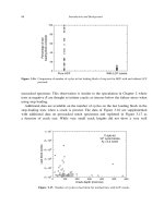
This function is shown schematically in Fig. 19.
Figure 19: Creep of open-ended pressure vessel subjected to constant internal pressure.
The situation is a bit more complicated if both the internal pressure and the material com-
pliance are time-dependent. It is incorrect simply to use the above equation with the value of
p
0
replaced by the value of p(t) at an arbitrary time, because the radial expansion at time t is
influenced by the pressure at previous times as well as the pressure at the current time.
The correct procedure is to “fold” the pressure and compliance functions together in a
convolution integral as was done in developing the Boltzman Superposition Principle. This
gives:
δ
r
(t)=
r
2
b

t
−∞
C

crp
(t − ξ)˙p(ξ) dξ (57)
Example 13
Let the internal pressure be a constantly increasing “ramp” function, so that p = R
p
t,withR
p
being
the rate of increase; then we have ˙p(ξ)=R
p
. Using the standard linear solid of Eqn. 55 for the creep
compliance, the stress is calculated from the convolution integral as
δ
r
(t)=
r
2
b

t
0

C
g
+(C
r
− C
g
)(1− e
−(t−ξ)/τ

)

R
p
dξ
=
r
2
b

R
p
tC
r
− R
p
τ (C
r
− C
g
)

1 −e
−t/τ

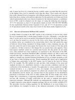
27
This function is plotted in Fig. 20, for a hypothetical material with parameters C
g
=1/3 × 10
5

psi
−1
,
C
r
=1/3 × 10
4
psi
−1
, b =0.2in,r =2in,τ =1month,andR
p
= 100 psi/month. Note that the
creep rate increases from an initial value (r
2
/b)R
p
C
g
to a final value (r
2
/b)R
p
C
r
as the glassy elastic
components relax away.
Figure 20: Creep δ
r
(t) of hypothetical pressure vessel for constantly increasing internal pressure.
When the pressure vessel has closed ends and must therefore resist axial as well as hoop

stresses, the radial expansion is δ
r
=(pr
2
/bE)[1− (ν/2)]. The extension of this relation to
viscoelastic material response and a time-dependent pressure is another step up in complexity.
Now two material descriptors, E and ν, must be modeled by suitable time-dependent functions,
and then folded into the pressure function. The superposition approach described above could
be used here as well, but with more algebraic complexity. The “viscoelastic correspondence
principle” to be presented in below is often more straightforward, but the superposition concept
is very important in understanding time-dependent materials response.
5.3 The viscoelastic correspondence principle
In elastic materials, the boundary tractions and displacements may depend on time as well
as position without affecting the solution: time is carried only as a parameter, since no time
derivatives appear in the governing equations. With viscoelastic materials, the constitutive or
stress-strain equation is replaced by a time-differential equation, which complicates the sub-
sequent solution. In many cases, however, the field equations possess certain mathematical
properties that permit a solution to be obtained relatively easily
5
. The “viscoelastic correspon-
dence principle” to be outlined here works by adapting a previously available elastic solution
to make it applicable to viscoelastic materials as well, so that a new solution from scratch is
unnecessary.
If a mechanics problem — the structure, its materials, and its boundary conditions of traction
and displacement — is subjected to the Laplace transformation, it will often be the case that
none of the spatial aspects of its description will be altered: the problem will appear the same, at
least spatially. Only the time-dependent aspects, namely the material properties, will be altered.
The Laplace-plane version of problem can then be interpreted as representing a stress analysis
5
E.H. Lee, “Viscoelasticity,” Handbook of Engineering Mechanics, W. Flugge, ed., McGraw-Hill, New York,

1962, Chap. 53.
28
problem for an elastic body of the same shape as the viscoelastic body, so that a solution for an
elastic body will apply to a corresponding viscoelastic body as well, but in the Laplace plane.
There is an exception to this correspondence, however: although the physical shape of the
body is unchanged upon passing to the Laplace plane, the boundary conditions for traction or
displacement may be altered spatially on transformation. For instance, if the imposed traction
is
ˆ
T =cos(xt), then
ˆ
T = s/(s
2
+x
2
); this is obviously of a different spatial form than the original
untransformed function. However, functions that can be written as separable space and time
factors will not change spatially on transformation:
ˆ
T (x, t)=f(x) g(t) ⇒
ˆ
T = f (x) g(s)
This means that the stress analysis problems whose boundary constraints are independent of
time or at worst are separable functions of space and time will look the same in both the actual
and Laplace planes. In the Laplace plane, the problem is then geometrically identical with an
“associated” elastic problem.
Having reduced the viscoelastic problem to an associated elastic one by taking transforms,
the vast library of elastic solutions may be used: one looks up the solution to the associated
elastic problem, and then performs a Laplace inversion to return to the time plane. The process
of viscoelastic stress analysis employing transform methods is usually called the “correspondence

principle”, which can be stated as the following recipe:
1. Determine the nature of the associated elastic problem. If the spatial distribution of the
boundary and body-force conditions is unchanged on transformation - a common occur-
rence - then the associated elastic problem appears exactly like the original viscoelastic
one.
2. Determine the solution to this associated elastic problem. This can often be done by
reference to standard handbooks
6
or texts on the theory of elasticity
7
.
3. Recast the elastic constants appearing in the elastic solution in terms of suitable viscoelas-
tic operators. As discussed in Section 5.1, it is often convenient to replace E and ν with
G and K, and then replace the G and K by their viscoelastic analogs:
E
ν

−→

G −→ G
K −→ K
4. Replace the applied boundary and body force constraints by their transformed counter-
parts:
ˆ
T ⇒
ˆ
T
ˆ
u ⇒
ˆ

u
where
ˆ
T and
ˆ
u are imposed tractions and displacements, respectively.
5. Invert the expression so obtained to obtain the solution to the viscoelastic problem in the
time plane.
6
For instance, W.C. Young, Ro ark’s Formulas for Stress and Strain, McGraw-Hill, Inc., New York, 1989.
7
For instance, S. Timoshenko and J.N. Goodier, The ory of Elasticity, McGraw-Hill, Inc., New York, 1951.
29
If the elastic solution contains just two time-dependent quantities in the numerator, such
as in Eqn. 54, the correspondence principle is equivalent to the superposition method of the
previous section. Using the pressure-vessel example, the correspondence method gives
δ
r
=
pr
2
C
b
→ δ
r
(s)=
r
2
b
pC

Since C = s
C
crp
, the transform relation for convolution integrals gives
δ
r
(t)=L
−1

r
2
b
sC
crp
· p

= L
−1

r
2
b
C
crp
· ˙p

=
r
2
b


t
−∞
C
crp
(t − ξ)˙p(ξ) dξ
as before. However, the correspondence principle is more straightforward in problems having a
complicated mix of time-dependent functions, as demonstrated in the following example.
Example 14
The elastic solution for the radial expansion of a closed-end cylindrical pressure vessel of radius r and
thickness b is
δ
r
=
pr
2
bE

1 −
ν
2

Following the correspondence-principle recipe, the associated solution in the Laplace plane is
δ
r
=
pr
2
bE


1 −
N
2

In terms of hydrostatic and shear response functions, the viscoelastic operators are:
E(s)=
9G(s)K(s)
3K(s)+G(s)
N(s)=
3K(s) − 2G(s)
6K(s)+2G(s)
In Example 12, we considered a PVC material at 75
◦
C that to a good approximation was elastic in
hydrostatic response and viscoelastic in shear. Using the standard linear solid model, we had
K = K
e
, G = G
r
+
(G
g
− G
r
)s
s +
1
τ
where K
e

=1.33 GPa, G
g
=800 MPA, G
r
=1.67 MPa, and τ =100 s.
For constant internal pressure p(t)=p
0
, p = p
0
/s. All these expressions must be combined, and the
result inverted. Maple commands for this problem might be:
define shear operator
> G:=Gr+((Gg-Gr)*s)/(s+(1/tau));
define Poisson operator
> N:=(3*K-2*G)/(6*K+2*G);
define modulus operator
> Eop:=(9*G*K)/(3*K+G);
define pressure operator
> pbar:=p0/s;
get d1, radial displacement (in Laplace plane)
> d1:=(pbar*r^2)*(1-(N/2))/(b*Eop);
read Maple library for Laplace transforms
> readlib(inttrans);
invert transform to get d2, radial displacement in real plane
> d2:=invlaplace(d1,s,t);
30
After some manual rearrangement, the radial displacement δ
r
(t)canbewrittenintheform
δ

r
(t)=
r
2
p
0
b

1
4G
r
+
1
6K

−

1
4G
r
−
1
4G
g

e
−t/τ
c

where the creep retardation time is τ

c
= τ(G
g
/G
r
). Continuing the Maple session:
define numerical parameters
> Gg:=800*10^6; Gr:=1.67*10^6; tau:=100; K:=1.33*10^9;
> r:=.05; b:=.005; p0:=2*10^5;
resulting expression for radial displacement
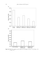
> d2;
- .01494 exp( - .00002088 t) + .01498
A log-log plot of this function is shown in Fig. 21. Note that for this problem the effect of the small
change in Poisson’s ratio ν during the transition is negligible in comparison with the very large change
in the modulus E, so that a nearly identical result would have been obtained simply by letting ν =
constant = 0.5. On the other hand, it isn’t appreciably more difficult to include the time dependence of
ν if symbolic manipulation software is available.
Figure 21: Creep response of PVC pressure vessel.
6 Additional References
1. Aklonis, J.J., MacKnight, W.J., and Shen, M., Introduction to Polymer Viscoelasticity,
Wiley-Interscience, New York, 1972.
2. Christensen, R.M., Theory of Viscoelasticity, 2nd ed., Academic Press, New York, 1982.
3. Ferry, J.D., Viscoelastic Properties of Polymers, 3rd ed., Wiley & Sons, New York, 1980.
4. Flugge, W., Viscoelasticity, Springer-Verlag, New York, 1975.
5. McCrum, N.G, Read, B.E., and Williams, G., Anelastic and Dielectric in Polymeric Solids,
Wiley & Sons, London, 1967. Available from Dover Publications, New York.
6. Tschoegl, N.W., The Phenomenological Theory of Linear Viscoelastic Behavior, Springer-
Verlag, Heidelberg, 1989.
31
7. Tschoegl, N.W., “Time Dependence in Materials Properties: An Overview,” M echanics of

Time-Dependent Materials, Vol. 1, pp. 3–31, 1997.
8. Williams, M.L., “Structural Analysis of Viscoelastic Materials,” AIAA Journal, p. 785,
May 1964.
7Problems
1. Plot the functions e
−t/τ
and 1 − e
−t/τ
versus log
10
t from t =10
−2
to t =10
2
.Havetwo
curves on the plot for each function, one for τ =1andoneforτ = 10.
2. Determine the apparent activation energy in (E
†
in Eqn. 2) for a viscoelastic relaxation in
which the initial rate is observed to double when the temperature is increased from 20
◦
C
to 30
◦
C. (Answer: E
†
= 51 kJ/mol.)
3. Determine the crosslink density N and segment molecular weight M
c
between crosslinks

for a rubber with an initial modulus E = 1000 psi at 20
◦
C and density 1.1 g/cm
3
.(Answer:
N = 944 mol/m
3
, M
c
= 1165 g/mol.)
4. Expand the exponential forms for the dynamic stress and strain

σ(t)=σ
∗
0
e
iωt
,(t)=
∗
0
e
iωt

and show that
E
∗
=
σ(t)
(t)
=

σ
0
cos δ

0
+ i
σ
0
sin δ

0
,
where δ is the phase angle between the stress and strain.
5. Using the relation
σ = E for the case of dynamic loading ((t)=
0
cos ωt) and S.L.S.
material response

E = k
e
+ k
1
s/(s +
1
τ
)

, solve for the time-dependent stress σ(t). Use
this solution to identify the steady-state components of the complex modulus E

∗
= E

+
iE

, and the transient component as well. Answer:
E
∗
=
k
1
1+ω
2
τ
2
e
−t/τ
+

k
e
+
k
1
ω
2
τ
2
1+ω

2
τ
2

cos ωt −

k
1
ωτ
1+ω
2
τ
2

sin ωt
6. For the Standard Linear Solid with parameters k
e
= 25, k
1
= 50, and τ
1
=1,plotE

and
E

versus log ω in the range 10
−2
< ωτ
1

< 10
2
. Also plot E

versus E

in this same range,
using ordinary rather than logarithmic axes and the same scale for both axes (Argand
diagram).
7. Show that the viscoelastic law for the “Voigt” form of the Standard Linear Solid (a spring
of stiffness k
v
=1/C
v
in parallel with a dashpot of viscosity η, and this combination in
series with another spring of stiffness k
g
=1/C
g
) can be written
 = Cσ, with C =


C
g
+
C
v
τ


s +
1
τ



where τ = η/k
v
.
32
Prob. 7
8. Show that the creep compliance of the Voigt SLS model of Prob. 7 is
C
crp
= C
g
+ C
v

1 − e
−t/τ

9. In cases where the stress rather than the strain is prescribed, the Kelvin model - a series
arrangement of Voigt elements - is preferable to the Wiechert model:
Prob. 9
where φ
j
=1/η
j
=˙

j
/σ
dj
and m
j
=1/k
j
= 
j
/σ
sj
Using the relations  = 
g
+

j

j
,
σ = σ
sj
+ σ
dj
, τ
j
= m
j
/φ
j
, show the associated viscoelastic constitutive equation to be:

 =


m
g
+

j
m
j
τ
j

s +
1
τ
j



σ
and for this model show the creep compliance to be:
C
crp
(t)=
(t)
σ
0
= m
g

+

j
m
j

1 − e
−t/τ
j

10. For a simple Voigt model (C
g
=0 in Prob. 7), show that the strain 
t+∆t
at time t +∆t
can be written in terms of the strain 
t
at time t and the stress σ
t
acting during the time
increment ∆t as

t+∆t
= C
v
σ
t

1 − e
−∆t/τ


+ 
t
e
−∆t/τ
Use this algorithm to plot the creep strain arising from a constant stress σ = 100 versus
log t =(1, 5) for C
v
=0.05 and τ = 1000.
11. Plot the strain response (t) to a load-unload stress input defined as
33
σ(t)=









0,t<1
1, 1 <t<4.5
−1, 4.5 <t<5
0,t>5
The material obeys the SLS compliance law (Eqn. 30) with C
g
=5,C
r
= 10, and τ =2.

12. Using the Maxwell form of the standard linear solid with k
e
= 10, k
1
= 100 and η = 1000:
a) Plot E
rel
(t)andE
crp
(t)=1/C
crp
(t)versuslogtime. b)Plot[E
crp
(t) − E
rel
(t)] versus
log time. c) Compare the relaxation time with the retardation time (the time when the
argument of the exponential becomes −1, for relaxation and creep respectively). Speculate
on why one is shorter than the other.
13. Show that a Wiechert model with two Maxwell arms (Eqn. 34) is equivalent to the second-
order ordinary differential equation
a
2
¨σ + a
1
˙σ + a
0
σ = b
2
¨ + b

1
˙ + b
0

where
a
2
= τ
1
τ
2
,a
1
= τ
1
+ τ
2
,a
0
=1
b
2
= τ
1
τ
2
(k
e
+ k
1

+ k
2
) ,b
1
= k
e
(τ
1
+ τ
2
)+k
1
τ
1
+ k
2
τ
2
,b
0
= k
e
14. For a viscoelastic material defined by the differential constitutive equation:
15¨σ +8˙σ + σ = 105¨ +34˙ + ,
write an expression for the relaxation modulus in the Prony-series form (Eqn. 36). (Answer:
E
rel
=1+2e
−t/3
+4e

−t/5
)
15. For the simple Maxwell element, verify that

t
0
E
rel
(ξ)D
crp
(t − ξ) dξ = t
16. Evaluate the Boltzman integral
σ(t)=

t
0
E
rel
(t − ξ)˙(ξ) dξ
to determine the response of the Standard Linear Solid to sinusoidal straining ((t)=
cos(ωt))
17. Derive Eqn. 48 by using the Arrhenius expression for relaxation time to subtract the log
relaxation time at an arbitrary temperature T from that at a reference temperature T
ref
.
18. Using isothermal stress relaxation data at various temperatures, shift factors have been
measured for a polyurethane material as shown in the table below:
34
T,
◦

C log
10
a
T
+5 -0.6
00
-5 0.8
-10 1.45
-15 2.30
-20 3.50
-25 4.45
-30 5.20
(a) Plot log a
T
vs. 1/T (
◦
K); compute an average activation energy using Eqn 48. (An-
swer: E
†
= 222 kJ/mol.)
(b) Plot log a
T
vs. T (
◦
C) and compare with WLF equation (Eqn. 50), with T
g
= −35
◦
C.
(Note that T

ref
=0= T
g
.)
19. After time-temperature shifting, a master relaxation curve at 0
◦
C for the polyurethane of
Prob. 18 gives the following values of E
rel
(t)atvarioustimes:
log(t, min) E
rel
(t), psi
-6 56,280
-5 22,880
-4 4,450
-3 957
-2 578
-1 481
0 480
(a) In Eqn. 36, choose k
e
= E
rel
(t = 0) = 480.
(b) Choose values of τ
j
to match the times given in the above table from 10
−6
to 10

−1
(a process called “collocation”).
(c) Determine appropriate values for the spring stiffnesses k
j
corresponding to each τ
j
so as to make Eqn. 36 match the experimental values of E
rel
(t). This can be done
by setting up and solving a sequence of linear algebraic equations with the k
j
as
unknowns:
6

j=1
k
j
e
−t
i
/τ
j
= E
rel
(t
i
) − k
e
,i=1, 6

Note that the coefficient matrix is essentially triangular, which facilitates manual
solution in the event a computer is not available.
(d) Adjust the value of k
1
so that the sum of all the spring stiffnesses equals the glassy
modulus E
g
=91, 100 psi.
(e) Plot the relaxation modulus predicted by the model from log t = −8to0.
20. Plot the relaxation (constant strain) values of modulus E and Poisson’s ratio ν for the
polyisobutylene whose dilatational and shear response is shown in Fig. 17. Assume S.L.S.
models for both dilatation and shear.
35
Prob. 19
21. The elastic solution for the stress σ
x
(x, y) and vertical deflection v(x, y) in a cantilevered
beam of length L and moment of inertia I, loaded at the free end with a force F,is
σ
x
(x, y)=
F (L − x)y
I
,v(x, y)=
Fx
2
6EI
(3L − x)
Determine the viscoelastic counterparts of these relations using both the superposition and
correspondence methods, assuming S.L.S. behavior for the material compliance (Eqn. 30).

Prob. 21
22. A polymer with viscoelastic properties as given in Fig. 17 is placed in a rigid circular die
and loaded with a pressure σ
y
= 1 MPa. Plot the transverse stress σ
x
(t)andtheaxial
strain 
y
(t)overlogt = −5to1. Theelasticsolutionis
σ
x
=
νσ
y
1 − ν
,
y
=
(1 + ν)(1 −2ν)
E(1 − ν)
σ
y
36
A Laplace Transformations
Basic definition:
Lf(t)=
f(s)=

∞

0
f(t) e
−st
dt
Fundamental properties:
L[c
1
f
1
(t)+c
2
f
2
(t)] = c
2
f
1
(s)c
1
f
2
(s)
L

∂f
∂t

= sf(s) − f (0
−
)

Some useful transform pairs:
f(t)
f(s)
u(t) 1/s
t
n
n!/s
n+1
e
−at
1/(s + a)
1
a
(1 − e
−at
) 1/s(s + a)
t
a
−
1
a
2
(1 − e
−at
) 1/s
2
(s + a)
Here u(t) is the Heaviside or unit step function, defined as
u(t)=


0,t<0
1,t≥ 0
The convolution integral:
Lf ·Lg =
f ·g = L


t
0
f(t − ξ) g(ξ) dξ

= L


t
0
f(ξ) g(t − ξ) dξ

37
Yield and Plastic Flow
David Roylance
Department of Materials Science and Engineering
Massachusetts Institute of Technology
Cambridge, MA 02139
October 15, 2001
Introduction
In our overview of the tensile stress-strain curve in Module 4, we described yield as a permanent
molecular rearrangement that begins at a sufficiently high stress, denoted σ
Y
in Fig. 1. The

yielding process is very material-dependent, being related directly to molecular mobility. It is
often possible to control the yielding process by optimizing the materials processing in a way
that influences mobility. General purpose polystyrene, for instance, is a weak and brittle plastic
often credited with giving plastics a reputation for shoddiness that plagued the industry for
years. This occurs because polystyrene at room temperature has so little molecular mobility
that it experiences brittle fracture at stresses less than those needed to induce yield with its
associated ductile flow. But when that same material is blended with rubber particles of suitable
size and composition, it becomes so tough that it is used for batting helmets and ultra-durable
children’s toys. This magic is done by control of the yielding process. Yield control to balance
strength against toughness is one of the most important aspects of materials engineering for
structural applications, and all engineers should be aware of the possibilities.
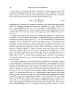
Figure 1: Yield stress σ
Y
as determined by the 0.2% offset method.
Another important reason for understanding yield is more prosaic: if the material is not
allowed to yield, it is not likely to fail. This is not true of brittle materials such as ceramics that
fracture before they yield, but in most of the tougher structural materials no damage occurs
before yield. It is common design practice to size the structure so as to keep the stresses in the
elastic range, short of yield by a suitable safety factor. We therefore need to be able to predict
1
when yielding will occur in general multidimensional stress states, given an experimental value
of σ
Y
.
Fracture is driven by normal stresses, acting to separate one atomic plane from another.
Yield, conversely, is driven by shearing stresses, sliding one plane along another. These two
distinct mechanisms are illustrated n Fig. 2. Of course, bonds must be broken during the sliding
associated with yield, but unlike in fracture are allowed to reform in new positions. This process
can generate substantial change in the material, even leading eventually to fracture (as in bending
a metal rod back and forth repeatedly to break it). The “plastic” deformation that underlies

yielding is essentially a viscous flow process, and follows kinetic laws quite similar to liquids.
Like flow in liquids, plastic flow usually takes place without change in volume, corresponding to
Poisson’s ratio ν =1/2.
Figure 2: Cracking is caused by normal stresses (a), sliding is caused by shear stresses (b).
Multiaxial stress states
The yield stress σ
Y
is usually determined in a tensile test, where a single uniaxial stress acts.
However, the engineer must be able to predict when yield will occur in more complicated real-life
situations involving multiaxial stresses. This is done by use of a yield criterion, an observation
derived from experimental evidence as to just what it is about the stress state that causes yield.
One of the simplest of these criteria, known as the maximum shear stress or Tresca criterion,
states that yield occurs when the maximum shear stress reaches a critical value τ
max
= k.The
numerical value of k for a given material could be determined directly in a pure-shear test, such
as torsion of a circular shaft, but it can also be found indirectly from the tension test as well. As
shown in Fig. 3, Mohr’s circle shows that the maximum shear stress acts on a plane 45
◦
away
from the tensile axis, and is half the tensile stress in magnitude; then k = σ
Y
/2.
In cases of plane stress, Mohr’s circle gives the maximum shear stress in that plane as half
the difference of the principal stresses:
τ
max
=
σ
p1

− σ
p2
2
(1)
2
Figure 3: Mohr’s circle construction for yield in uniaxial tension.
Example 1
Using σ
p1
= σ
θ
= pr/b and σ
p2
= σ
z
= pr/2b in Eqn. 1, the shear stress in a cylindrical pressure vessel
with closed ends is
1
τ
max,θ z
=
1
2

pr
b
−
pr
2b


=
pr
4b
where the θz subscript indicates a shear stress in a plane tangential to the vessel wall. Based on this, we
might expect the pressure vessel to yield when
τ
max,θ z
= k =
σ
Y
2
which would occur at a pressure of
p
Y
=
4bτ
max,θ z
r
?
=
2bσ
Y
r
However, this analysis is in error, as can be seen by drawing Mohr’s circles not only for the θz plane but
for the θr and rz planes as well as shown in Fig. 4.
Figure 4: Principal stresses and Mohr’s circle for closed-end pressure vessel
The shear stresses in the θr planeareseentobetwicethoseintheθz plane, since in the θr plane
the second principal stress is zero:
τ
max,θ r

=
1
2

pr
b
− 0

=
pr
2b
Yield will therefore occur in the θr plane at a pressure of bσ
Y
/r, half the value needed to cause yield in
the θz plane. Failing to consider the shear stresses acting in this third direction would lead to a seriously
underdesigned vessel.
Situations similar to this example occur in plane stress whenever the principal stresses in the
xy plane are of the same sign (both tensile or both compressive). The maximum shear stress,
1
See Mo dule 6.
3
which controls yield, is half the difference between the principal stresses; if they are both of the
same sign, an even larger shear stress will occur on the perpendicular plane containing the larger
of the principal stresses in the xy plane.
This concept can be used to draw a “yield locus” as shown in Fig. 5, an envelope in σ
1
-σ
2
coordinates outside of which yield is predicted. This locus obviously crosses the coordinate
axes at values corresponding to the tensile yield stress σ

Y
. In the I and III quadrants the
principal stresses are of the same sign, so according to the maximum shear stress criterion yield
is determined by the difference between the larger principal stress and zero. In the II and IV
quadrantsthelocusisgivenbyτ
max
= |σ
1
−σ
2
|/2=σ
Y
/2, so σ
1
−σ
2
= const; this gives straight
diagonal lines running from σ
Y
on one axis to σ
Y
on the other.
Figure 5: Yield locus for the maximum-shear stress criterion.
Example 2
Figure 6: (a) Circular shaft subjected to simultaneous twisting and tension. (b) Mohr’s circle
construction.
A circular shaft is subjected to a torque of half that needed to cause yielding as shown in Fig. 6; we now
ask what tensile stress could be applied simultaneously without causing yield.
4
A Mohr’s circle is drawn with shear stress τ = k/2 and unknown tensile stress σ. Using the Tresca

maximum-shear yield criterion, yield will occur when σ is such that
τ
max
= k =


σ
2

2
+

k
2

2
σ =
√
3 k
The Tresca criterion is convenient to use in practice, but a somewhat better fit to experi-
mental data can often be obtained from the “von Mises” criterion, in which the driving force for
yield is the strain energy associated with the deviatoric components of stress. The von Mises
stress (also called the equivalent or effective stress) is defined as
σ
M
=

1
2
[(σ

x
− σ
y
)
2
+(σ
x
− σ
z
)
2
+(σ
y
− σ
z
)
2
+6(τ
xy
+ τ
yz
+ τ
xz
)]
In terms of the principal stresses this is
σ
M
=

1

2
[(σ
1
− σ
2
)
2
+(σ
1
− σ
3
)
2
+(σ
2
− σ
3
)
2
]
where the stress differences in parentheses are proportional to the maximum shear stresses on
the three principal planes
2
. (Since the quantities are squared, the order of stresses inside the
parentheses is unimportant.) The Mises stress can also be written in compact form in terms of
the second invariant of the deviatoric stress tensor Σ
ij
:
σ
M

=

3Σ
ij
Σ
ij
/2(2)
It can be shown that this is proportional to the total distortional strain energy in the material,
and also to the shear stress τ
oct
on the “octahedral” plane oriented equally to the 1-2-3 axes.
The von Mises stress is the driving force for damage in many ductile engineering materials, and
is routinely computed by most commercial finite element stress analysis codes.
The value of von Mises stress σ
M,Y
needed to cause yield can be determined from the tensile
yield stress σ
Y
, since in tension at the yield point we have σ
1
= σ
Y
,σ
2
= σ
3
=0. Then
σ
M,Y
=


1
2
[(σ
Y
− 0)
2
+(σ
Y
−0)
2
+(0− 0)
2
]=σ
Y
Hence the value of von Mises stress needed to cause yield is the same as the simple tensile yield
stress.
The shear yield stress k can similarly be found by inserting the principal stresses corre-
sponding to a state of pure shear in the Mises equation. Using k = σ
1
= −σ
3
and σ
2
=0,we
have

1
2
[(k − 0)

2
+(k + k)
2
+(0−k)
2
]=

6k
2
2
= σ
Y
k =
σ
Y
√
3
2
Some authors use a factor other than 1/2 within the radical. This is immaterial, since it will be absorbed by
the calculation of the critical value of σ
M
.
5