InTech-Climbing and walking robots towards new applications Part 1 doc

Preface




The research field of robotics has been contributing widely and significantly to in-
dustrial applications for assembly, welding, painting, and transportation for a long
time. Meanwhile, the last decades have seen an increasing interest in developing
and employing mobile robots for industrial inspection, conducting surveillance,
urban search and rescue, military reconnaissance and civil exploration.

As a special potential sub-group of mobile technology, climbing and walking ro-
bots can work in unstructured environments. They are useful devices adopted in a
variety of applications such as reliable non-destructive evaluation (NDE) and di-
agnosis in hazardous environments, welding and manipulation in the construction
industry especially of metallic structures, and cleaning and maintenance of high-
rise buildings. The development of walking and climbing robots offers a novel so-
lution to the above-mentioned problems, relieves human workers of their hazard-
ous work and makes automatic manipulation possible, thus improving the techno-
logical level and productivity of the service industry.

Currently there are several different kinds of kinematics for motion on horizontal
and vertical surfaces: multiple legs, sliding frames, wheeled and chain-track vehi-
cles. All of the above kinematics modes have been presented in this book. For ex-
ample, six-legged walking robots and humanoid robots are multiple-leg robots; the
climbing cleaning robot features a sliding frame; while several other mobile proto-
types are contained in a wheeled and chain-track vehicle.

Generally a light-weight structure and efficient manipulators are two important is-
sues in designing climbing and walking robots. Even though significant progress
has been made in this field, the technology of climbing and walking robots is still a
challenging topic which should receive special attention by robotics research. For
example, note that previous climbing robots are relatively large. The size and
weight of these prototypes is the choke point. Additionally, the intelligent technol-
ogy in these climbing robots is not well developed.
VI
With the advancement of technology, new exciting approaches enable us to render
mobile robotic systems more versatile, robust and cost-efficient. Some researchers
combine climbing and walking techniques with a modular approach, a reconfigur-
able approach, or a swarm approach to realize novel prototypes as flexible mobile
robotic platforms featuring all necessary locomotion capabilities.

The purpose of this book is to provide an overview of the latest wide-range
achievements in climbing and walking robotic technology to researchers, scientists,
and engineers throughout the world. Different aspects including control simula-
tion, locomotion realization, methodology, and system integration are presented
from the scientific and from the technical point of view.

This book consists of two main parts, one dealing with walking robots, the second
with climbing robots. The content is also grouped by theoretical research and ap-
plicative realization. Every chapter offers a considerable amount of interesting and
useful information. I hope it will prove valuable for your research in the related
theoretical, experimental and applicative fields.

Editor
Dr. Houxiang Zhang

University of Hamburg
Germany
















1
Mechanics and Simulation
of Six-Legged Walking Robots
Giorgio Figliolini and Pierluigi Rea
DiMSAT, University of Cassino
Cassino (FR), Italy
1. Introduction

Legged locomotion is used by biological systems since millions of years, but wheeled
locomotion vehicles are so familiar in our modern life, that people have developed a sort of
dependence on this form of locomotion and transportation. However, wheeled vehicles
require paved surfaces, which are obtained through a suitable modification of the natural
environment. Thus, walking machines are more suitable to move on irregular terrains, than
wheeled vehicles, but their development started in long delay because of the difficulties to
perform an active leg coordination.
In fact, as reported in (Song and Waldron, 1989), several research groups started to study
and develop walking machines since 1950, but compactness and powerful of the existent
computers were not yet suitable to run control algorithms for the leg coordination. Thus,
ASV (Adaptive-Suspension-Vehicle) can be considered as the first comprehensive example
of six-legged walking machine, which was built by taking into account main aspects, as
control, gait analysis and mechanical design in terms of legs, actuation and vehicle structure.
Moreover, ASV belongs to the class of “statically stable” walking machines because a static
equilibrium is ensured at all times during the operation, while a second class is represented
by the “dynamically stable” walking machines, as extensively presented in (Raibert, 1986).
Later, several prototypes of six-legged walking robots have been designed and built in the
world by using mainly a “technical design” in the development of the mechanical design
and control. In fact, a rudimentary locomotion of a six-legged walking robot can be achieved
by simply switching the support of the robot between a set of legs that form a tripod.
Moreover, in order to ensure a static walking, the coordination of the six legs can be carried
out by imposing a suitable stability margin between the ground projection of the center of
gravity of the robot and the polygon among the supporting feet.
A different approach in the design of six-legged walking robots can be obtained by referring
to biological systems and, thus, developing a biologically inspired design of the robot. In
fact, according to the “technical design”, the biological inspiration can be only the trivial
observation that some insects use six legs, which are useful to obtain a stable support during
the walking, while a “biological design” means to emulate, in every detail, the locomotion of
a particular specie of insect. In general, insects walk at several speeds of locomotion with a
Source: Climbing & Walking Robots, Towards New Applications, Book edited by Houxiang Zhang,

ISBN 978-3-902613-16-5, pp.546, October 2007, Itech Education and Publishing, Vienna, Austria
O
pen Access Database www.i-techonline.co
m
Climbing & Walking Robots, Towards New Applications
2
variety of different gaits, which have the property of static stability, but one of the key
characteristics of the locomotion control is the distribution.
Thus, in contrast with the simple switching control of the “technical design”, a distributed
gait control has to be considered according to a “biological design” of a six-legged walking
robot, which tries to emulate the locomotion of a particular insect. In other words, rather
than a centralized control system of the robot locomotion, different local leg controllers can
be considered to give a distributed gait control.
Several researches have been developed in the world by referring to both “cockroach
insect”, or Periplaneta Americana, as reported in (Delcomyn and Nelson, 2000; Quinn et al.,
2001; Espenschied et al., 1996), and “stick insect”, or Carausius Morosus, as extensively
reported in (Cruse, 1990; Cruse and Bartling, 1995; Frantsevich and Cruse, 1997; Cruse et al.,
1998; Cymbalyuk et al., 1998; Cruse, 2002; Volker et al., 2004; Dean, 1991 and 1992).
In particular, the results of the second biological research have been applied to the
development of TUM (Technische-Universität-München) Hexapod Walking Robot in order
to emulate the locomotion of the Carausius Morosus, also known as stick insect. In fact, a
biological design for actuators, leg mechanism, coordination and control, is much more
efficient than technical solutions.
Thus, TUM Hexapod Walking Robot has been designed as based on the stick insect and
using a form of the Cruse control for the coordination of the six legs, which consists on
distributed leg control so that each leg may be self-regulating with respect to adjacent legs.
Nevertheless, this walking robot uses only Mechanism 1 from the Cruse model, i.e. “A leg is
hindered from starting its return stroke, while its posterior leg is performing a return
stroke”, and is applied to the ispilateral and adjacent legs.
TUM Hexapod Walking Robot is one of several prototypes of six-legged walking robots,

which have been built and tested in the world by using a distributed control according to
the Cruse-based leg control system. The main goal of this research has been to build
biologically inspired walking robots, which allow to navigate smooth and uneven terrains,
and to autonomously explore and choose a suitable path to reach a pre-defined target
position. The emulation of the stick insect locomotion should be performed through a
straight walking at different speeds and walking in curves or in different directions.
Therefore, after some quick information on the Cruse-based leg controller, the present
chapter of the book is addressed to describe extensively the main results in terms of
mechanics and simulation of six-legged walking robots, which have been obtained by the
authors in this research field, as reported in (Figliolini et al., 2005, 2006, 2007). In particular,
the formulation of the kinematic model of a six-legged walking robot that mimics the
locomotion of the stick insect is presented by considering a biological design. The algorithm
for the leg coordination is independent by the leg mechanism, but a three-revolute ( 3R )
kinematic chain has been assumed to mimic the biological structure of the stick insect. Thus,
the inverse kinematics of the 3R has been formulated by using an algebraic approach in
order to reduce the computational time, while a direct kinematics of the robot has been
formulated by using a matrix approach in order to simulate the absolute motion of the
whole six-legged robot.
Finally, the gait analysis and simulation is presented by analyzing the results of suitable
computer simulations in different walking conditions. Wave and tripod gaits can be
observed and analyzed at low and high speeds of the robot body, respectively, while a
transient behaviour is obtained between these two limit conditions.
Mechanics and Simulation of Six-Legged Walking Robots
3
2. Leg coordination
The gait analysis and optimization has been obtained by analyzing and implementing the
algorithm proposed in (Cymbalyuk et al., 1998), which was formulated by observing in
depth the walking of the stick insect and it was found that the leg coordination for a six-
legged walking robot can be considered as independent by the leg mechanism.
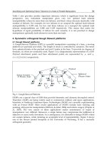
Referring to Fig. 1, a reference frame GĻ (xĻ

G
yĻ
G
zĻ
G
) having the origin GĻ coinciding with the
projection on the ground of the mass center G of the body of the stick insect and six
reference frames O
Si
(x
Si
y
Si
z
Si
) for i = 1,…,6, have been chosen in order to analyze and
optimize the motion of each leg tip with the aim to ensure a suitable static stability during
the walking.
Thus, in brief, the motion of each leg tip can be expressed as function of the parameters
Si
p
ix
and s
i
, where
Si
p
ix
gives the position of the leg tip in O
Si

(x
Si
y
Si
z
Si
) along the x-axis for the
stance phase and s
i
∈{0 ; 1} indicates the state of each leg tip, i.e. one has: s
i
= 0 for the swing
phase and s
i
= 1 for the stance phase, which are both performed within the range [PEP
i
,
AEP
i
], where PEP
i
is the Posterior-Extreme-Position and AEP
i
is the Anterior-Extreme-Position
of each tip leg. In particular, L is the nominal distance between PEP
0
and AEP
0
.
The trajectory of each leg tip during the swing phase is assigned by taking into account the

starting and ending times of the stance phase.
d
3
d
2
L
d
1
d
0
O
S4
y
S4
x
S4
O
S5
y
S5
x
S5
O
S6
y
S6
x
S6
y
S2

l
1
l
3
O
S2
O
S3
x
S3
O
S1
y
S1
x
S1
PEP
05
AEP
05
l
0
y
S3
x
S2
G'
x
'
G

y'
G
forward
motion
Fig. 1. Sketch and sizes of the stick insect: d
1
= 18 mm, d
2
= 20 mm, d
3
= 15 mm, l
1
= l
3
= 24
mm, L = 20 mm, d
0
= 5 mm, l
0
= 20 mm
Climbing & Walking Robots, Towards New Applications
4
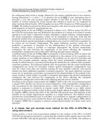
3. Leg mechanism
A three-revolute (3R) kinematic chain has been chosen for each leg mechanism in order to
mimic the leg structure of the stick insect through the coxa, femur and tibia links, as shown
in Fig. 2.
A direct kinematic analysis of each leg mechanism is formulated between the moving frame
O
Ti
(x

Ti
y
Ti
z
Ti
) of the tibia link and the frame O
0i
(x
0i
y
0i
z
0i
), which is considered as fixed
frame before to be connected to the robot body, in order to formulate the overall kinematic
model of the six-legged walking robot, as sketched in Fig. 3.
In particular, the overall transformation matrix
0i
Ti
M
between the moving frame O
Ti
(x
Ti
y
Ti
z
Ti
) and the fixed frame O
0i

(x
0i
y
0i
z
0i
) is given by
0
11 12 13
0
0
21 22 23
123
0
31 32 33
(, , )
000 1
i
ix
i
i
iy
Ti i i i
i
iz
rrr p
rrr p
rrr p
ϑϑ ϑ
ªº

«»
«»
=
«»
«»
«»
¬¼
M
.
(1)
This matrix is obtained as product between four transformation matrices, which relate the
moving frame of the tibia link with the three typical reference frames on the revolute joints
of the leg mechanism.
Thus, each entry r
jk
of
0i
Ti
M
for j,k = 1, 2, 3 and the Cartesian components of the position
vector p
i
in frame O
0i
(x
0i
y
0i
z
0i

) are given by
11 0 1 21 1 31 1 0
12 3 0 2 0 1 2 3 0 1 2 0 2
22 1 2 3 1 2 3
32 3 0 2 0 1 2 3 0 1 2 0 2
13 3 0 1 2 0
cs; c; ss
s(ss ccc)c(ccs sc)
scs ssc
s(cs scc)c(scs cc)
c(ccc s
iii
ii iiiii i
iii iii
ii iiiii i
iii
rrr
r
r
r
r
αϑ ϑ ϑα
ϑαϑ αϑϑ ϑαϑϑ αϑ
ϑϑϑ ϑϑ ϑ
ϑαϑ αϑϑ ϑαϑϑ αϑ
ϑαϑϑ α
==−=−
=−− +
=− −
=++ +

=−
2301202
23 1 2 3 1 2 3
33 3012 02 3012 02
0
3012 02 3012 023
01 2 02
s)s(ccs sc)
scc sss
c(scc cs)s(scs cc)
[c (c c c s s ) s (c c s s c )]
(c c c s s )
ii ii i
iii iii
iii iiii i
i
ixiii iiii i
ii i
r
r
pa
ϑϑαϑϑαϑ
ϑϑϑ ϑϑϑ
ϑαϑϑ αϑ ϑαϑϑ αϑ
ϑαϑϑ αϑ ϑαϑϑ αϑ
αϑϑ αϑ
−+
=−
=− + + −
=−−++

+−
()()
2011
0
3123 123 122 11
0
3012 02 3012 023
01 2 02 2 011
cc
scc sss sc s
[ c (s c c c s ) s (s c s c c )]
(s c c c s ) s c
i
i
iy iii iii ii i
i
iziii iiii i
ii i i
aa
pa a a
p
a
aa
αϑ
ϑϑϑ ϑϑϑ ϑϑ ϑ
ϑαϑϑ αϑ ϑαϑϑ αϑ
αϑϑ αϑ αϑ
+
=−++
=− + + − +

−−−
(2)
where
ϑ
1i
,
ϑ
2i
and
ϑ
3i
are the variable joint angles of each leg mechanism
( i = 1,…,6 ),
α
0
is the angle of the first joint axis with the axis z
0i
, and a
1
, a
2
and a
3
are the
lengths of the coxa, femur and tibia links, respectively.
Mechanics and Simulation of Six-Legged Walking Robots
5
The inverse kinematic analysis of the leg mechanism is formulated through an algebraic
approach. Thus, when the Cartesian components of the position vector p
i

are given in the
frame O
Fi
(x
Fi
y
Fi
z
Fi
), the variable joint angles
ϑ
1i
,
ϑ
2i
and
ϑ
3i
( i = 1,…,6) can be expressed as
1
atan2 ( , )
Fi Fi
iiyix
pp
ϑ
=
(3)
and
333
atan2(s , c )

iii
ϑϑϑ
=
,
(4)
where
2222 2222
11 23
3
23
2
33
()()() 2()()
c
2
s1c
Fi Fi Fi Fi Fi
ix iy iz ix iy
i
ii
pppaappaa
aa
ϑ
ϑϑ
+++− +−−
=
=± −
,
(5)
x

0i
y
0i
≡ y
Fi
z
0i
h
i
d
i
L
i
AEP
0i
PEP
0i
L/
2
L/
2
y
Si
x
Si
z
Si
2i
ϑ
1i

ϑ

3i
ϑ
a
1
a
2
a
3
α

0
robot body
p
i
z
Ti
x
Ti
y
Ti
forward
motion
z
Fi
Si
p
i
h

T
tibia link
coxa link
femur link
swing phase
stance phase
Fig. 2. A 3R leg mechanism of the six-legged walking robot
Climbing & Walking Robots, Towards New Applications
6
and, in turn, by
222
atan2(s , c )
iii
ϑϑϑ
=
,
(6)
where
(
)
()
()
22
33 2 33
2
22
23 233
22 33
2
33

s()() c
s
2c
sc
c
s
Fi Fi Fi
iix iy iz i
i
i
Fi
iz i i
i
i
apppaa
aa aa
paa
a
ϑϑ
ϑ
ϑ
ϑϑ
ϑ
ϑ
+++
=−
++
++
=−
.

(7)
Therefore, the Eqs. (1-7) let to formulate the overall kinematic model of the six-legged
walking robot, as proposed in the following.
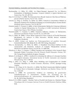
4. Kinematic model of the six-legged walking robot
Referring to Figs. 2 and 3, the kinematic model of a six-legged walking robot is formulated
through a direct kinematic analysis between the moving frame O
Ti
(x
Ti
y
Ti
z
Ti
) of the tibia link
and the inertia frame O (X Y Z).
In general, a six-legged walking robot has 24 d.o.f.s, where 18 d.o.f.s are given by
ϑ
1i
,
ϑ
2i
and
ϑ
3i
(i = 1,…,6) for the six 3R leg mechanisms and 6 d.o.f.s are given by the robot body,
which are reduced in this case at only 1 d.o.f. that is given by X
G
in order to consider the
pure translation of the robot body along the X-axis.
Thus, the equation of motion X

G
(t) of the robot body is assigned as input of the proposed
algorithm, while
ϑ
1i
(t),
ϑ
2i
(t) and
ϑ
3i
(t) for i = 1,…,6 are expressed through an inverse
kinematic analysis of the six 3R leg mechanisms when the equation of motion of each leg tip
is given and the trajectory shape of each leg tip during the swing phase is assigned.
In particular, the transformation matrix M
G
of the frame G (x
G
y
G
z
G
) on the robot body with
respect to the inertia frame O (X Y Z ) is expressed as
()
100
010
001
000 1
GX

GY
GG
GZ
X
p
p
p
ªº
«»
«»
=
«»
«»
¬¼
M
,
(8)
where p
GX
= X
G
, p
GY
= 0 and p
GZ
= h
G
.
The transformation matrix
G

B
i
M of the frame O
Bi
(x
Bi
y
Bi
z
Bi
) on the robot body with respect to
the frame G (x
G
y
G
z
G
) is expressed by
Mechanics and Simulation of Six-Legged Walking Robots
7
0
0
0 1 0
1 0 0
for = 1, 2, 3
0 0 1 0
0 0 0 1
01 0
1 0 0
for = 4, 5, 6

0 0 1 0
0 0 0 1
i
G
Bi
i
d
l
i
d
l
i

ªº
°
«»
−
°
«»
°
«»
°
«»
°¬ ¼
=
®
−
ªº
°
«»

°
−
«»
°
«»
°
«»
°
¬¼
¯
M
(9)
where l
1
= l
4
= – l
0
, l
2
= l
5
= 0, l
3
= l
6
= l
0
.
Therefore, the direct kinematic function of the walking robot is given by

123 123
()() (),,, ,,
G
GBi0i
TiGiii G Bi 0i Tiiii
XX
ϑϑ ϑ ϑϑ ϑ
=M M MMM
(10)
where
Bi
0i
=MI
, being I the identity matrix.
The joint angles of the leg mechanisms are obtained through an inverse kinematic analysis.
In particular, the position vector
()
Si
i
tp of each leg tip in the frame O
Si
(x
Si
y
Si
z
Si
), as shown
in Fig.2, is expressed in the next section along with a detailed motion analysis of the leg tip.
Moreover, the transformation matrix

B
i
Si
M
is given by

3
3
01 0
1 0 0
for = 1, 2, 3
0 0 1
0 0 0 1
0 1 0
1 0 0
for = 4, 5, 6
0 0 1
0 0 0 1
i
i
i
Bi
Si
i-
i-
i
L
d
i
h

L
d
i
h

−
ªº
°
«»
°
«»
°
«»
−
°
«»
°¬ ¼
=
®
ªº
°
«»
°
−−
«»
°
«»
−
°
«»

°
¬¼
¯
M
(11)
where L
1
= l
1
– l
0
, L
2
= 0 and L
3
= l
3
– l
0
with L
i
shown in Fig.2.
Finally, the position of each leg tip in the frame O
Fi
(x
Fi
y
Fi
z
Fi

) is given by
0
0
() ()
Fi Fi i Bi Si
iiBiSii
tt=p MMM p (12)
where the matrix
0
F
i
i
M
can be easily obtained by knowing the angle
α
0
.
Climbing & Walking Robots, Towards New Applications
8
Therefore, substituting the Cartesian components of ()
Fi
i
tp in Eqs. (3), (5) and (7), the joint
angles
ϑ
1i
,
ϑ
2i
and

ϑ
3i
(i = 1,…,6) can be obtained.
x
B3
y
B3
z
B3
x
B2
y
B2
z
B2
x
01
y
01
z
01
y
G
x
G
z
G
G
PEP
1

AEP
2
PEP
2
AEP
3
PEP
3
forward
motion
x
03
z
03
y
03
x
02
y
02
z
02
z
B1
y
B1
x
B1
y
S3

z
S3
x
S3
y
S2
z
S2
x
S2
y
S1
x
S1
Y
X
Z
O
robot body
p
G
z
S1
AEP
1
h
G
Gƍ
Fig. 3. Kinematic scheme of the six-legged walking robot
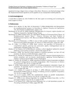
5. Motion analysis of the leg tip

The gait of the robot is obtained by a suitable coordination of each leg tip, which is
fundamental to ensure the static stability of the robot during the walking. Thus, a typical
motion of each leg tip has to be imposed through the position vector
Si
p
i
(t), even if a variable
gait of the robot can be obtained according to the imposed speed of the robot body.
Referring to Figs. 2 to 4, the position vector
Si
p
i
(t) of each leg tip can be expressed as
() 1
T
Si Si Si Si
iixiyiz
t ppp
ªº
=
¬¼
p
(13)
in the local frame O
Si
(x
Si
y
Si
z

Si
) for i = 1,…,6, which is considered as attached and moving
with the robot body.
Referring to Fig. 4, the x-coordinate
Si
p
ix
of vector
Si
p
i
(t) is given by the following system of
difference equations
() ()
()
() ()
for 1
for 0
ix r i
Si
ix
ix p i
tV t
tt
tV t
pt s
p
pt s
−
+Δ

+
Δ=

°
=
®
Δ=
°
¯
(14)
where V
r
is the velocity of the tip of each leg mechanism during the retraction motion of the
stance phase, even defined power stroke, since producing the motion of the robot body, and
V
p
is the velocity along the robot body of the tip of each leg mechanism during the
protraction motion of the swing phase, even defined return stroke, since producing the
forward motion of the leg mechanism.
Mechanics and Simulation of Six-Legged Walking Robots
9
h
T
z
Si
x
Si
O
Si
V

p
V
p
V
r
< V
p
V
Si
p
i
L/2 L/2
AEP
0
PEP
0
V
G
= V
r
swing phase
stance phase
(t
0
)
i
(t
f
)
i

Fig. 4. Trajectory and velocities of the tip of each leg mechanism during the stance and
swing phases
Parameter s
i
defines the state of the i-th leg, which is equal to 1 for the retraction state, or
stance phase, and equal to 0 for the protraction state, or swing phase.
Both velocities V
p
and V
r
are supposed to be constant and identical for all legs, for which the
speed V
G
of the center of mass of the robot body is equal to V
r
because of the relative
motion. In fact, during the stance phase (power stroke), each tip leg moves back with
velocity V
r
with respect to the robot body and, consequentially, this moves ahead with the
same velocity. Thus, the function
()
Si
ix
pt of Eq. (2) for i = 1, …, 6 is linear periodic function.
Moreover, it is quite clear that the static stability of the six-legged walking robot is obtained
only when V
r
(=V
G

) < V
p
, because the robot body cannot move forward faster than its legs
move in the same direction during the swing phase. Likewise,
Si
p
iy
is equal to zero in order
to obtain a vertical planar trajectory, while
Si
p
iz
is given by
0
0
()
()
()
0for 1
sin for 0
i
Si
i
iz
Ti
ii
f
t
t
t

s
p
tt
hs
tt
π
=

°
§·
=
−
®
=
¨¸
°
¨¸
−
©¹
¯
(15)
where h
T
is the amplitude of the sinusoid and time t is the general instant, while
0
i
t and
i
f
t

are the starting and ending times of the swing phase, respectively.
Times
0
i
t and
i
f
t take into account the mechanism of the leg coordination, which give a
suitable variation of AEP
i
and PEP
i
in order to ensure the static stability.
Thus, referring to the time diagrams of V
G
in Fig. 5, the time diagrams of Figs. 6 to 8 have
been obtained. In particular, Fig. 5 shows the time diagrams of the robot speeds V
G
= 0.05,
0.1, 0.5 and 0.9 mm/s for the case of constant acceleration a = 0.002 mm/s
2
. Thus, the
transient periods t = 25, 50, 250 and 450 s for the speeds V
G
= 0.05, 0.1, 0.5 and 0.9 mm/s of
the robot body are obtained respectively before to reach the steady-state condition at
Climbing & Walking Robots, Towards New Applications
10
constant speed. The time diagrams of Figs. 6 to 8 show the horizontal x-displacement, the x-
component of the velocity, the vertical z-displacement, the z-component of the velocity, the

magnitude of the velocity and the trajectory of the leg tip 1 (front left leg) of the six-legged
walking robot. Thus, before to analyze in depth the time diagrams of Figs. 6 to 8, it may be
useful to refer to the motion analysis of the leg tip and to remind that the protraction speed
V
p
along the axis of the robot body has been assigned as constant and equal to 1 mm/s for
the swing phase of the leg tip. In other words, only the retraction speed V
r
can be changed
since related and equal to the robot speed V
G
, which is assigned as input data.
Consequently, the range time during the stance phase between two consecutive steps of
each leg can vary in significant way because of the different imposed speeds V
r
= V
G
, while
the time range to perform the swing phase of each leg is almost the same because of the
same speed V
p
and similar overall x-displacements.
In particular, Fig. 6 show computer simulations between the time range 200 - 340 s, which is
after the transient periods of 25 and 50 s for V
G
= 0.05 and 0.1 mm/s, respectively.
Thus, both x-component of the velocity, protraction speed V
p
= 1 mm/s and retraction speed
V

r
= V
G
= 0.05 and 0.1 mm/s, are constant versus time. Instead, Figs. 7 and 8 show two
computer simulations between the time ranges of 0 - 400 s and 200 - 600 s, which are greater
than the transient periods of 250 and 450 s for the robot speeds V
G
of 0.5 and 0.9 mm/s,
respectively. Thus, the transient behavior of the velocities is also shown at the constant
acceleration of 0.002 mm/s
2
. In fact, during these time ranges of 250 and 450 s, the
protraction speed V
p
is always constant and equal to 1 mm/s, while the retraction speed V
r
varies linearly according to the constant acceleration, before to reach the steady-state
condition and to equalize the speed V
G
of the robot body. The same effect is also shown by
the time diagrams of Figs. 7e and 8e, which show the magnitude of the velocity.
Moreover, single loop trajectories are shown in the simulations of Figs. 6e and 6m, because
one step only is performed by the leg mechanism 1, while multi-loop trajectories are shown
in the simulations of Figs. 7f and 8f, because 3 (three) and 7 (seven) steps are performed by
the leg mechanism 1, respectively. The variation of the step length is also evident in Figs. 7f
and 8f because of the influence mechanisms for the leg coordination.
Fig. 5. Time diagrams of the robot body speed for a constant acceleration a = 0.002 mm/s
2
and V
G

= 0.05, 0.1, 0.5 and 0.9 mm/s
Mechanics and Simulation of Six-Legged Walking Robots
11
Fig. 6. Computer simulations for the motion analysis of the leg tip of a six-legged walking
robot when V
G
= 0.05 and 0.1 [mm/s]: a) and g) horizontal x-displacement; b) and h)
vertical z-displacement; c) and i) x-component of the velocity; d) and l) z-component
of the velocity; e) and m) planar trajectory in the xz-plane; f) and n) magnitude of the
velocity
Climbing & Walking Robots, Towards New Applications
12
Fig. 7. Computer simulations within the time range 0 - 400 s for the motion analysis of the
leg tip when V
G
= 0.5 [mm/s]: a) horizontal x-displacement; b) x-component of the
velocity; c) vertical z-displacement; d) z-component of the velocity; e) magnitude of
the velocity; f ) planar trajectory in the xz-plane
Mechanics and Simulation of Six-Legged Walking Robots
13
Fig. 8. Computer simulations within the time range 200-600 s for the motion analysis of the
leg tip when V
G
= 0.9 [mm/s]: a) horizontal x-displacement; b) x-component of the
velocity; c) vertical z-displacement; d) z-component of the velocity; e) magnitude of
the velocity; f ) planar trajectory in the xz-plane
Climbing & Walking Robots, Towards New Applications
14
6. Gait analysis
A suitable overall algorithm has been formulated as based on the kinematic model of the

six-legged walking robot and on the leg tip motion of each leg mechanism. This algorithm
has been implemented in a Matlab program in order to analyze the absolute gait of the six-
legged walking robot, which mimics the behavior of the stick insect, for different speeds of
the robot body. Thus, the absolute gait of the robot is analyzed by referring to the results of
suitable computer simulations, which have been obtained by running the proposed
algorithm. In particular, the results of three computer simulations are reported in the
following in the form of time diagrams of the z and x-displacements of the tip of each leg
mechanism. These three computer simulations have been obtained for three different input
parameters in terms of speed and acceleration of the robot body.
The same constant acceleration a = 0.002 mm/s
2
has been considered along with three
different speeds V
G
= 0.05, 0.1 and 0.9 mm/s of the center of mass of the robot body, as
shown in the time diagram of Fig. 5. Of course, the transient time before to reach the steady-
state condition is different for the three simulations because of the same acceleration which
has been imposed. Moreover, the protraction speed V
p
along the axis of the robot body has
been assigned equal to 1 mm/s for the swing phase. Thus, only the retraction speed V
r
of
the tip of each leg mechanism is changed since related and equal to the speed V
G
of the
center of mass of the robot body. Consequently, the range time during the stance phase
between two consecutive steps of each leg varies in significant way because of the different
imposed speeds V
r

= V
G
, while the time range to perform the swing phase of each leg is
almost the same because of the same speed V
p
and similar overall x-displacements.
The time diagrams of the z and x-displacements of each leg of the six-legged walking robot
are shown in Figs. 9 to 11, as obtained for a = 0.002 mm/s
2
and V
G
= 0.05 mm/s. It is
noteworthy that the maximum vertical stroke of the tip of each leg mechanism is always
equal to 10 mm, while the maximum horizontal stroke is variable and different for the tip of
each leg mechanism according to the leg coordination, which takes into account the static
stability of the six-legged walking robot. However, these horizontal strokes of the tip of each
leg mechanism are quite centered around 0 mm and similar to the nominal stroke L = 24
mm, which is considered between the extreme positions AEP
0
and PEP
0
.
Moreover, the horizontal x-displacements are represented through liner periodic functions,
where the slope of the line for the swing phase is constant and equal to the speed V
p
= 1
mm/s, while the slope of the line for the stance phase is variable according to the assigned
speed V
G
, as shown in Figs. 9, 10 and 11 for V

G
= 0.05, 01 and 0.9 mm/s, respectively.
In particular, referring to Fig. 11, the slopes of both linear parts of the linear periodic
function of the x-displacement are almost the same, as expected, because the protraction
speed of 1 mm/s is almost equal to the retraction speed of 0.9 mm/s.
Moreover, three different gait typologies of the six-legged walking robot can be observed in
the three simulations, which are represented in the diagrams of Figs. 9 to 11.
In particular, the simulation of Fig. 9 show a wave gait of the robot, which is typical at low
speeds and that can be understood with the aid of the sketch of Fig. 12a. In fact, referring to
the first peak of the diagram of leg 1 of Fig. 9, which takes place after 400 s and, thus, after
the transient time before to reach the steady-state condition of 0.05 mm/s, the second leg to
move is leg 5 and, then, leg 3. Thus, observing in sequence the peaks of the z-displacements
of the six legs, after leg 3, it is the time of the leg 4 and, then, leg 2 in order to finish with leg
6, as sketched in Fig. 12a, before to restart the wave gait.
Mechanics and Simulation of Six-Legged Walking Robots
15
0 200 400 600 800 1000 1200 1400 1600 1800
0
5
10
time [s] (Leg 1)
z
S1
0 200 400 600 800 1000 1200 1400 1600 1800
0
5
10
time [s] (Leg 2)
z
S2

0 200 400 600 800 1000 1200 1400 1600 1800
0
5
10
time [s] (Leg 3)
z
S3
0 200 400 600 800 1000 1200 1400 1600 1800
0
5
10
time [s] (Leg 4)
z
S4
0 200 400 600 800 1000 1200 1400 1600 1800
0
5
10
time [s] (Leg 5)
z
S5
0 200 400 600 800 1000 1200 1400 1600 1800
0
5
10
time [s] (Leg 6)
z
S6
a)
0 200 400 600 800 1000 1200 1400 1600 1800

-20
0
20
time [s] (Leg 1)
x
S1
0 200 400 600 800 1000 1200 1400 1600 1800
-20
0
20
time [s] (Leg 2)
x
S2
0 200 400 600 800 1000 1200 1400 1600 1800
-20
0
20
time [s] (Leg 3)
x
S3
0 200 400 600 800 1000 1200 1400 1600 1800
-20
0
20
time [s] (Leg 4)
x
S4
0 200 400 600 800 1000 1200 1400 1600 1800
-20
0

20
time [s] (Leg 5)
x
S5
0 200 400 600 800 1000 1200 1400 1600 1800
-20
0
20
time [s] (Leg 6)
x
S6
b)
Fig. 9. Displacements of the leg tip for V
G
= 0.05 mm/s and a = 0.002 mm/s
2
: a) vertical z-
displacement; b) horizontal x-displacement
Climbing & Walking Robots, Towards New Applications
16
0 200 400 600 800 1000 1200 1400 1600 1800
0
5
10
time [s] (Leg 1)
z
S1
0 200 400 600 800 1000 1200 1400 1600 1800
0
5

10
time [s] (Leg 2)
z
S2
0 200 400 600 800 1000 1200 1400 1600 1800
0
5
10
time [s] (Leg 3)
z
S3
0 200 400 600 800 1000 1200 1400 1600 1800
0
5
10
time [s] (Leg 4)
z
S4
0 200 400 600 800 1000 1200 1400 1600 1800
0
5
10
time [s] (Leg 5)
z
S5
0 200 400 600 800 1000 1200 1400 1600 1800
0
5
10
time [s] (Leg 6)

z
S6
a)
0 200 400 600 800 1000 1200 1400 1600 1800
-20
0
20
time [s] (Leg 1)
x
S1
0 200 400 600 800 1000 1200 1400 1600 1800
-20
0
20
time [s] (Leg 2)
x
S2
0 200 400 600 800 1000 1200 1400 1600 1800
-20
0
20
time [s] (Leg 3)
x
S3
0 200 400 600 800 1000 1200 1400 1600 1800
-20
0
20
time [s] (Leg 4)
x

S4
0 200 400 600 800 1000 1200 1400 1600 1800
-20
0
20
time [s] (Leg 5)
x
S5
0 200 400 600 800 1000 1200 1400 1600 1800
-20
0
20
time [s] (Leg 6)
x
S6
b)
Fig. 10. Displacements of the leg tip for V
G
= 0.1 mm/s and a = 0.002 mm/s
2
: a) vertical z-
displacement; b) horizontal x-displacement
Mechanics and Simulation of Six-Legged Walking Robots
17
0 200 400 600 800 1000 1200 1400 1600 1800
0
5
10
time [s] (Leg 1)
z

S1
0 200 400 600 800 1000 1200 1400 1600 1800
0
5
10
time [s] (Leg 2)
z
S2
0 200 400 600 800 1000 1200 1400 1600 1800
0
5
10
time [s] (Leg 3)
z
S3
0 200 400 600 800 1000 1200 1400 1600 1800
0
5
10
time [s] (Leg 4)
z
S4
0 200 400 600 800 1000 1200 1400 1600 1800
0
5
10
time [s] (Leg 5)
z
S5
0 200 400 600 800 1000 1200 1400 1600 1800

0
5
10
time [s] (Leg 6)
z
S6
a)
0 200 400 600 800 1000 1200 1400 1600 1800
-20
0
20
time [s] (Leg 1)
x
S1
0 200 400 600 800 1000 1200 1400 1600 1800
-20
0
20
time [s] (Leg 2)
x
S2
0 200 400 600 800 1000 1200 1400 1600 1800
-20
0
20
time [s] (Leg 3)
x
S3
0 200 400 600 800 1000 1200 1400 1600 1800
-20

0
20
time [s] (Leg 4)
x
S4
0 200 400 600 800 1000 1200 1400 1600 1800
-20
0
20
time [s] (Leg 5)
x
S5
0 200 400 600 800 1000 1200 1400 1600 1800
-20
0
20
time [s] (Leg 6)
x
S6
b)
Fig. 11. Displacements of the leg tip for V
G
= 0.9 mm/s and a = 0.002 mm/s
2
: a) vertical z-
displacement; b) horizontal x-displacement
Climbing & Walking Robots, Towards New Applications
18
1 2 3
4

5
6
1 2 3
4
5
6
1 2 3
4
5
6
a) b) c)
Fig. 12. Typical gaits of a six-legged walking robot: a) wave; b) transient gait; c) tripod
The simulation of Fig. 10 show the case of a particular gait of the robot, which is not wave
and neither tripod, as it will be explained in the following. The sequence of the steps for this
particular gait can be also understood with the aid of the sketch of Fig. 12b. This gait
typology of the six-legged walking robot can be considered as a transient gait between the
two extreme cases of wave and tripod gaits.
In fact, the tripod gait can be observed by referring to the time diagrams reported in Fig. 11.
The tripod gait can be understood by analyzing the sequence of the peaks of the
z-displacements for the tip of each leg mechanism and with the aid of the sketch of Fig. 12c.
The tripod gait is typical at high speeds of the robot body. In fact, the simulation of Fig. 11
has been obtained for V
G
= 0.9 mm/s, which is almost the maximum speed (V
p
= 1 mm/s)
reachable by the robot before to fall down because of the loss of the static stability. In
particular, legs 1, 5 and 3 move together to perform a step and, then, legs 4, 2 and 6 move
together to perform another step of the six-legged walking robot. Both steps are performed
with a suitable phase shift according to the input speed.

7. Absolute gait simulation
This formulation has been implemented in a Matlab program in order to analyze the
performances of a six-legged walking robot during the absolute gait along the X-axis of the
inertia frame O ( XYZ).
Figures 13 and 14 show two significant simulations for the wave and tripod gaits, which
have been obtained by running the proposed algorithm for V
G
= 0.05 mm/s and V
G
= 0.9
mm/s, respectively. In particular, six frames for each simulation are reported along with the
inertia frame, which can be observed on the right side of each frame, as indicating the
starting position of the robot. Thus, the robot moves toward the left side by performing a
transient motion at constant acceleration a = 0.002 mm/s
2
before to reach the steady-state
condition with a constant speed.
In particular, for the wave gait cycle of Fig. 13, all leg tips are on the ground in Fig. 13a and
leg tip 4 performs a swing phase in Fig. 13b before to touch the ground in Fig. 13c. Then, leg
tip 2 performs a swing phase in Fig. 13d before to touch the ground in Fig. 13e and, finally,
leg tip 6 performs a swing phase in Fig. 13f.
Similarly, for the tripod gait cycle of Fig. 14, all leg tips are on the ground in Figs. 14a, 14c
and 14e. Leg tips 4-2-6 perform a swing phase in Fig. 14b and 14f between the swing phase
performed by the leg tips 1-5-3 in Fig. 14d.
Mechanics and Simulation of Six-Legged Walking Robots
19
a) b)
c) d)
e) f)
Fig. 13. Animation of a wave gait along the X-axis for V

G
= 0.05 mm/s and a = 0.002 mm/s
2
:
a), c) and e), all leg tips are on the ground; b) leg tip 4 performs a swing phase; d) leg
tip 2 performs a swing phase; f) leg tip 6 performs a swing phase
Climbing & Walking Robots, Towards New Applications
20
a) b)
c) d)
e) f)
Fig. 14. Animation of a tripod gait along the X-axis for V
G
= 0.9 mm/s and a = 0.002 mm/s
2
:
a), c) and e), all leg tips are on the ground; b) leg tips 4-2-6 perform a swing phase;
d) leg tips 1-5-3 perform a swing phase; f) leg tips 4-2-6 perform a swing phase
Mechanics and Simulation of Six-Legged Walking Robots
21
8. Conclusions
The mechanics and locomotion of six-legged walking robots has been analyzed by
considering a simple “technical design”, in which the biological inspiration is only given by
the trivial observation that some insects use six legs to obtain a static walking, and
considering a “biological design”, in which we try to emulate, in every detail, the
locomotion of a particular specie of insect, as the “cockroach” or “stick” insects.
In particular, as example of the mathematical approach to analyze the mechanics and
locomotion of six-legged walking robots, the kinematic model of a six-legged walking robot,
which mimics the biological structure and locomotion of the stick insect, has been
formulated according to the Cruse-based leg control system.

Thus, the direct kinematic analysis between the moving frame of the tibia link and the
inertia frame that is fixed to the ground has been formulated for the six 3R leg mechanisms,
where the joint angles have been expressed through an inverse kinematic analysis when the
trajectory of each leg tip is given. This aspect has been considered in detail by analyzing the
motion of each leg tip of the six-legged walking robot in the local frame, which is considered
as attached and moving with the robot body.
Several computer simulations have been reported in the form of time diagrams of the
horizontal and vertical displacements along with the horizontal and vertical components of
the velocities for a chosen leg of the robot. Moreover, single and multi-loop trajectories of a
leg tip have been shown for different speeds of the robot body, in order to put in evidence
the effects of the Cruse-based leg control system, which ensures the static stability of the
robot at different speeds by adjusting the step length of each leg during the walking.
Finally, the gait analysis and simulation of the six-legged walking robot, which mimics the
locomotion of the stick insect , have been carried out by referring to suitable time diagrams
of the z and x-displacements of the six legs, which have shown the extreme typologies of the
wave and tripod gaits at low and high speeds of the robot body, respectively.
9. References
Song, S.M. & Waldron, K.J., (1989). Machines That Walk: the Adaptive Suspension Vehicle, MIT
Press, ISBN 0-262-19274-8, Cambridge, Massachusetts.
Raibert, M.H., (1986). Legged Robots That Balance, MIT Press, ISBN 0-262-18117-7, Cambridge,
Massachusetts.
Delcomyn, F. & Nelson, M. E. (2000). Architectures for a biomimetic hexapod robot, Robotics
and Autonomous Systems, Vol. 30, pp.5–15.
Quinn, R. D., Nelson, G. M., Bachmann, R. J., Kingsley, D. A., Offi J. & Ritzmann R. E.,
(2001). Insect Designs for Improved Robot Mobility, Proceedings of the 4
th
International Conference on Climbing and Walking Robots, Berns and Dillmann (Eds),
Professional Engineering Publisher, London, pp. 69-76.
Espenschied, K.S., Quinn, R.D., Beer, R.D. & Chiel H.J., (1996). Biologically based distributed
control and local reflexes improve rough terrain locomotion in a hexapod robot,

Robotics and Autonomous Systems, Vol. 18, pp. 59-64.
Cruse, H., (1990). What mechanisms coordinate leg movement in walking arthropods ?,
Trends in Neurosciences, Vol. 13, pp. 15-21.
Cruse, H. & Bartling, Ch., (1995). Movement of joint angles in the legs of a walking insect,
Carausius morosus, J. Insect Physiology, Vol. 41 (9), pp.761-771.
Climbing & Walking Robots, Towards New Applications
22
Frantsevich, F. & Cruse, H., (1997). The stick insect, Obrimus asperrimus (Phasmida,
Bacillidae) walking on different surfaces, J. of Insect Physiology, Vol. 43 (5), pp.447-
455.
Cruse, H., Kindermann, T., Schumm, M., Dean, J. and Schmitz, J., (1998). Walknet - a
biologically inspired network to control six-legged walking, Neural Networks,
Vol.11, pp. 1435-1447.
Cymbalyuk, G.S., Borisyuk, R.M., Müeller-Wilm, U. & Cruse, H., (1998). Oscillatory network
controlling six-legged locomotion. Optimization of model parameters, Neural
Networks, Vol. 11, pp. 1449-1460.
Cruse, H., (2002). The functional sense of central oscillations in walking, Biological
Cybernetics, Vol. 86, pp. 271-280.
Volker, D., Schmitz, J. & Cruse, H., (2004). Behaviour-based modelling of hexapod
locomotion: linking biology and technical application, Arthropod Structure &
Development, Vol. 33, pp. 237–250.
Dean, J., (1991). A model of leg coordination in the stick insect, Carausius morosus. I.
Geometrical consideration of coordination mechanisms between adjacent legs.
Biological Cybernetics, Vol. 64, pp. 393-402.
Dean, J., (1991). A model of leg coordination in the stick insect, Carausius morosus. II.
Description of the kinematic model and simulation of normal step patterns.
Biological Cybernetics, Vol. 64, pp. 403-411.
Dean, J., (1992). A model of leg coordination in the stick insect, Carausius morosus, III.
Responses to perturbations of normal coordination, Biological Cybernetics, Vol. 66,
pp. 335-343.

Dean, J., (1992). A model of leg coordination in the stick insect, Carausius morosus, IV.
Comparison of different forms of coordinating mechanisms, Biological Cybernetics,
Vol. 66, pp. 345-355.
Mueller-Wilm, U., Dean, J., Cruse, H., Weidermann, H.J., Eltze, J. & Pfeiffer, F., (1992).
Kinematic model of a stick insect as an example of a six-legged walking system,
Adaptive Behavior, Vol. 1 (2), pp. 155–169.
Figliolini, G. & Ripa, V., (2005). Kinematic Model and Absolute Gait Simulation of a Six-
Legged Walking Robot, In: Climbing and Walking Robots, Manuel A. Armada &
Pablo González de Santos (Ed), pp. 889-896, Springer, ISBN 3-540-22992-6, Berlin.
Figliolini, G., Rea, P. & Ripa, V., (2006). Analysis of the Wave and Tripod Gaits of a Six-
Legged Walking Robot, Proceedings of the 9
th
International Conference on Climbing and
Walking Robots and Support Technologies for Mobile Machines, pp. 115-122, Brussels,
Belgium, September 2006.
Figliolini, G., Rea, P. & Stan, S.D., (2006). Gait Analysis of a Six-Legged Walking Robot
When a Leg Failure Occurs, Proceedings of the 9
th
International Conference on Climbing
and Walking Robots and Support Technologies for Mobile Machines, pp. 276-283,
Brussels, Belgium, September 2006.
Figliolini, G., Stan, S.D. & Rea, P. (2007). Motion Analysis of the Leg Tip of a Six-Legged
Walking Robot, Proceedings of the 12
th
IFToMM World Congress, Besançon (France),
paper number 912.
2
Attitude and Steering Control of the
Long Articulated Body Mobile Robot KORYU
Edwardo F. Fukushima and Shigeo Hirose

Tokyo Institute of Technology
Tokyo, Japan
1. Introduction
Many types of mobile robots have been considered so far in the robotics community,
including wheeled, crawler track, and legged robots. Another class of robots composed of
many articulations/segments connected in series, such as “Snake-like robots”, “Train-like
Robots” and “Multi-trailed vehicles/robots” has also been extensively studied. This
configuration introduces advantageous characteristics such as high rough terrain
adaptability and load capacity, among others. For instance, small articulated robots can
tread through rubbles and be useful for inspection, search-and-rescue tasks, while larger
and longer ones can be used for maintenance tasks and transportation of material, where
normal vehicles cannot approach. Some ideas and proposal appeared in the literature, to
build such big robots; many related studies concerning this configuration have been
reported (Waldron, Kumar & Burkat, 1987; Commissariat A I’Energie Atomique, 1987;
Burdick, Radford & Chirikjian, 1993; Tilbury, Sordalen & Bushnell, 1995; Shan and Koren,
1993; Nilsson, 1997; Migads and Kyriakopoulos, 1997). However, very few real mechanical
implementations have been reported.
An actual mechanical model of an “Articulated Body Mobile Robot” was introduced by
Hirose & Morishima in 1988, and two mechanical models of articulated body mobile robot
called KORYU (KR for short) have been developed and constructed, so far. KORYU was
mainly developed for use in fire-fighting reconnaissance and inspection tasks inside nuclear
reactors. However, highly terrain adaptive motions can also be achieved such as; 1) stair
climbing, 2) passing over obstacles without touching them, 3) passing through meandering
and narrow paths, 4) running over uneven terrain, and 5) using the body’s degrees of
freedom not only for “locomotion”, but also for “manipulation”. Hirose and Morishima
(1990) performed some basic experimental evaluations using the first model KR-I (a 1/3
scale model compared to the second model KR-II, shown in Fig. 1(a)-(c). Improved control
strategies have been continuously studied in order to generate more energy efficient
motions.
This chapter addresses two fundamental control strategies that are necessary for long

articulated body mobile robots such as KORYU to perform the many inherent motion
capabilities cited above. The control issue can be divided in two independent tasks, namely
1) Attitude Control and 2) Steering Control. The underlying concept for the presented
O
pen Access Database www.i-techonline.co
m
Source: Climbing & Walking Robots, Towards New Applications, Book edited by Houxiang Zhang,
ISBN 978-3-902613-16-5, pp.546, October 2007, Itech Education and Publishing, Vienna, Austria