InTech-Climbing and walking robots towards new applications Part 3 pdf

60 Climbing & Walking Robots, Towards New Applications
;2,1,
1
d
d
*
d
d
d
d
1
4
4
4
3
3210
2
3210
1
3210
0
0
0
=+
¨
©
§
+=
i
z

y
x
t
tt
z
y
x
i
P
i
P
i
P
iiii
iiiiiiii
i
P
i
P
i
P
θ
θθ
θ
θθ
AQAAA
AAQAAAAAQA




;4,3
,
1
d
d
*
d
d
d
d
d
d
d
d
d
d
1
4
4
4
3
321
9
3
8
2
7
10
2
321

9
3
8
2
7
10
1
321
9
3
8
2
7
10
9
3
321
9
3
8
2
7
10
8
2
321
9
3
8
2

7
10
7
1
321
9
3
8
2
7
10
0
0
0
=
¸
¸
¹
·
++
++
+
¨
¨
©
§
=
i
z
y

x
tt
tt
tt
z
y
x
i
P
i
P
i
P
i
iiii
i
iiii
i
iiiiiiii
iiiiiiii
i
P
i
P
i
P
θ
θ
θ
θ

θθ
θθ
θθ
θθ
AQAAAAAAAAQAAAAA
AAAQAAAAAAAAQAAA
AAAAAQAAAAAAAAQA



;6,5
,
1
d
d
d
d
d
d
d
d
d
d
d
d
1
4
4
4
3

321
12
3
11
2
10
10
2
321
12
3
11
2
10
10
1
321
12
3
11
2
10
10
12
3
321
12
3
11
2

10
10
11
2
321
12
3
11
2
10
10
10
1
321
12
3
11
2
10
10
0
0
0
=
¸
¸
¹
·
+++
+++

++
¨
¨
©
§
=
i
z
y
x
tt
tt
tt
z
y
x
i
P
i
P
i
P
i
iiii
i
iiii
i
iiiiiiii
iiiiiiii
i

P
i
P
i
P
θ
θ
θ
θ
θθ
θθ
θθ
θθ
AQAAAAAAAAQAAAAA
AAAQAAAAAAAAQAAA
AAAAAQAAAAAAAAQA



Modular Walking Robots 61
4. Force Distribution in Displacement Systems of Walking Robots
The system builds by the terrain on which the displacement is done and the walking robot
which has three legs in the support phase is statically determinate.
When it leans upon four (or more) feet, it turns in a statically indeterminate system.
The problem of determination of reaction force components is made in simplifying
assumption, namely the stiffness of the walking robot mechanical structure and terrain.
For establishing the stable positions of a walking robot it is necessary to determine the forces
distribution in the shifting mechanisms. In the case of a uniform and rectilinear movement
of the walking robot on a plane and horizontal surface, the reaction forces do not have the
tangential components, because the applied forces are the gravitational forces only.

Determination of the real forces distribution in the shifting mechanisms of a walking
locomotion system which moves in rugged land at low speed is necessary for the analysis of
stability. The position of a walking system depends on the following factors:
• the configuration of walking mechanisms;
• the masses of component elements and their positions of gravity centers;
• the values of friction coefficients between terrain and feet;
• the shape of terrain surface.
• the stiffness of terrain;
The active surface of the foot is relatively small and it is considered that the reaction force is
applied in the gravity center of this surface. The reaction force represents the resultant of the
elementary forces, uniformly distributed on the foot sole surface. The gravity center of the
foot active surface is called theoretical contact point.
To calculate the components of reaction forces, namely:
• normal component N , perpendicular on the surface of terrain in the theoretical
contact point;
• tangential component
T
, or coulombian frictional force, comprised in the tangent
plane at terrain surface in the theoretical contact point,
it is necessary to determine the stable positions of walking robots (Ion I., Simionescu I. &
Curaj A.,. 2002), (Ion I. & Stefanescu D.M., 1999).
The magnitude of T vector cannot be greater than the product of the magnitude of the
normal component
N by the frictional coefficient μ between foot sole and terrain. If this
magnitude is greater than the friction force, then the foot slips down along the support
surface to the stable position, where the magnitudes of this component decrease under the
above-mentioned limit.
Therefore, the problem of determining the stable position of a walking robot upon some
terrain has not a unique solution. For every foot is available a field which covers all contact
points in which the condition T

≤μN is true. The equal sign corresponds to the field’s
boundary.
The complex behavior of the earth cannot be described than by an idealization of its
properties. The surface of terrain which the robot walks on is defined in respect to a fixed
62 Climbing & Walking Robots, Towards New Applications
coordinates system Oξηζ annexed to the terrain, by the parametrical equations ξ = ξ(u, v); η
= η(u, v); ζ = ζ(u, v), implicit equation F(ξ,η,ζ) = 0, or explicit equation ζ = f(ξ,η).
These real, continuous and uniform functions with continuous first partial and ordinary
derivative, establish a biunivocal correspondence between the points of support surface and
the ordered pairs (u, v), where {u, v}
∈ R. Not all partial first order derivatives are null, and
not all Jacobians
),(
),(
;
),(
),(
;
),(
),(
vuD
D
vuD
D
vuD
D
ξ
ζ
ζ
η

η
ξ
are simultaneous null.
On the entire surface of the terrain, the equation expressions may be unique or may be
multiple, having the limited domains of validity.
Fig. 8. The Hartenberg – Denavit coordinate systems and the reaction force components
The normal component
i
N of reaction force at the P
i
contact point of the leg i with the
terrain is positioned by the direction cosine:
;cos
222
iii
i
i
CBA
A
++
=
α
;cos
222
iii
i
i
CBA
B
++

=
β
,cos
222
iii
i
i
CBA
C
++
=
γ
with respect to the fixed coordinate axes system, where:
.;;
ii
ii
i
ii
ii
i
ii
ii
i
vv
uu
C
vv
uu
B
vv

uu
A
ii
ii
ii
ii
ii
ii
∂
∂η
∂
∂ξ
∂
∂η
∂
∂ξ
∂
∂ξ
∂
∂ζ
∂
∂ξ
∂
∂ζ
∂
∂ζ
∂
∂η
∂
∂ζ

∂
∂η
===
The tangential component of reaction force, i.e. the friction force, is comprised in the tangent
plane at the support surface. The equation of the tangent plane in the point P
i
(ξ
Pi
, η
Pi
, ζ
Pi
) is
Modular Walking Robots 63
,0=
∂
∂ζ
∂
∂η
∂
∂ξ
∂
∂ζ
∂
∂η
∂
∂ξ
ζ−ζη−ηξ−ξ
i
i

i
i
i
i
i
i
i
i
i
i
Pi
i
Pi
i
Pi
i
vvv
uuu
or: ξ
i
A
i
+ η
i
B
i
+ ζ
i
C
i

- ξ
Pi
A
i
- η
Pi
B
i
- ζ
Pi
C
i
= 0.
The straight-line support of the friction force is included in the tangent plane:
,
i
Pi
i
i
Pi
i
i
Pi
i
nml
ζ−ζ
=
η−η
=
ξ−ξ

therefore: A
i
l
i
+ B
i
m
i
+ C
i
n
i
= 0.
If the surface over which the robot walked is plane, it is possible that the robot may slip to
the direction of the maximum slope.
Generally, the sliding result is a rotational motion superposed on a translational one. The
instantaneous axis has an unknown position.
Let us consider
rrr
V
U
γ
ζ
=
β
−η
=
α
−ξ
coscoscos

the equation of instantaneous axis under canonical form, with respect to the fixed coordinate
axes system The components of speed of the point P
i
, on the fixed coordinate axes system
with OZ axis identical with the instantaneous axis, are:
,;;
0
VVjXViYV
ZYX
=ω=ω−=
The projections of the P
i
point speed on the axes of fixed system Oξηζ are:
Z
Y
X
V
V
V
V
V
V
R=
ς
η
ξ
,
where R is the matrix of rotation in space.
The carrier straight line of P
i

point speed, i.e. of the tangential component of reaction force,
has the equations
,
ζηξ
ζ
=
η−η
=
ξ
−
ξ
VVV
PiPi
and is contained in the tangent plane to the terrain surface in the point P
i
:
V
ξ
l + V
η
m + V
ζ
n = 0.
To determine the stable position of the walking robot which leans upon n legs, on some
shape terrain, it is necessary to solve a nonlinear system, which is formed by:
- the transformation matrix equation
64 Climbing & Walking Robots, Towards New Applications
11
4
4

4
3210
0
0
0
Pi
Pi
Pi
iiii
Pi
Pi
Pi
Z
Y
X
Z
Y
X
AAAAA=
,
where:
A is the transformation matrix of coordinate of a point from the system O
0
X
0
Y
0
Z
0
of the

robot platform to the system O
ξηζ;
A
i
is the Denavit – Hartenberg transformation matrix of coordinates of a point from the
system O
i+1
X
i+1
Y
i+1
Z
i+1
of the element (i) to the system O
i
X
i
Y
i
Z
i
of the element (i-1) (Denavit
J. & Hartenberg R.S., 1955), (Uicker J.J.jr., Denavit J., Hartenberg R.S., 1965):
- the balance equations
¦¦
==
=+=+
n
i
R

n
i
i
MMFR
i
1
)(
1
,0;0
(8)
which expressed the equilibrium of the forces and moments system, which acted on the
elements of walking robot.
The
F and M are the wrench components of the forces and moments which represent the
robot load, including the own weight.
The unknowns of the system are:
• the coordinates X
T
, Y
T
, Z
T
and direction cosines cos α
T
, cos β
T
, cos γ
T
which define
the platform position with respect to the terrain:

• the normal
i
N and the tangential
i
T , ni ,1= , components of the reaction forces;
• the direction numbers l
i
, m
i
, n
i
, ni ,1= , of the tangential components;
• the position parameters U, V, cos α, cos β, cos γ of the instantaneous axis;
• the magnitude of the V
0
/ω ratio, where V
0
is the translational instantaneous speed
of the hardening structure (Okhotsimski D.E. & Golubev I., 1984). The system is
compatible for n = 3 support points.
If the number of feet which are simultaneous in the support phase is larger than three the
system is undetermined static and is necessary to take into consideration the deformations
of the mechanical structure of the walking robot and terrain. In case of a quadrupedal
walking robot, the hardening configuration is a six fold hyperstatical structure. To
determinate the force distribution, one must use a specific method for indeterminate static
systems.
The canonical equations in stress method are (Buzdugan Gh., 1980):
δ
11
x

1
+ δ
12
x
2
+ … + δ
16
x
6
= – δ
10
;
δ
21
x
1
+ δ
22
x
2
+ … + δ
26
x
6
= – δ
20
; (9)
. . . . . .
Modular Walking Robots 65
δ

61
x
1
+ δ
62
x
2
+ … + δ
66
x
6
= – δ
60
;
where:
δ
ij
is the displacement along the O
i
X
i
direction of stress owing to unit load which acts
on the direction and in application point of the O
i
X
j
;
δ
i0
is the displacement along the X

i
direction of stress owing to the external load when
O
i
X
j
= 0, 6,1=i :
6,1,dd
4
1
2
0
4
1
1
0
0
=+=
¦
³
¦
³
==
ix
EI
mM
x
EI
mM
q

y
yiy
p
y
yiy
i
δ
;
;6,1,6,1,d
dd
dd
dd
dd
4
1
3
4
1
2
4
1
1
4
1
3
4
1
2
4
1

1
4
1
3
4
1
2
4
1
1
==+
+++
+++
+++
++=
¦
³
¦
³
¦
³
¦
³
¦
³
¦
³
¦
³
¦

³
¦
³
=
==
==
==
==
jix
GI
mM
x
GI
mM
x
GI
mM
x
GI
mM
x
GI
mM
x
GI
mM
x
GI
mM
x

GI
mM
x
GI
mM
q
z
zizi
q
z
zizi
p
z
zizi
q
y
yiyi
q
y
yiyi
p
y
yiyi
q
x
xixi
q
x
xixi
p

x
xixi
ij
δ
GI
xi
, 3,1=i , are the torsion stiffness of the legs elements lowers, middles and uppers
respectively;
EI
yi
and EI
zi
, 3,1=i , are the bend stiffness of the legs elements lowers, middles and uppers
respectively;
M are the bending moments in basic system which is loaded with basic charge;
m are the bending moments in the basic system loaded with the unit charge.
The definite integrals
³
=
b
a
xMmI d
are calculated by the Simpson method:
]))([(
6
bbaababa
mMmMmmMM
ab
I ++++
−

=
.
To calculate the m
xi
, m
yi
, m
zi
, M
xi
, M
yi
, M
zi
, 6,1=i , seven systems are used (Fig. 8), namely:
• the system S
0
, where the single load is G, and X
i
= 0, 6,1=i ;
66 Climbing & Walking Robots, Towards New Applications
• the systems S
i
, where the single load is X
i
= 1,
6,1=i
.
The remaining unknowns, namely x
i

, 12,7=i , are calculated from the equations (9). The
normal and tangential components of the reaction forces are calculated as function of the
positions of tangent planes on the terrain surface at the support points.
The following hypotheses are considered as true:
• the stiffnesses of the legs are much less than the robot’s platform stiffness;
• the four legs are identically.
• the cross sections of the leg’s elements are constant.
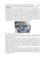
In Fig. 9, a modular walking robot with six legs is shown. The hardening structure of this
robot is a 12-fold hyperstatical structure.
Fig. 9. The reaction force components in the support points of the modular walking robot
5. Movement of Walking Robots
Part of the characteristic parameters of the walking robot may change widely enough when
using it as a transportation mean. For instance, the additional loads on board, change the
positions of the gravity centers and the inertia moments of the module’s platforms.
Environmental factors such as the wind or other elements may bias the robot, and their
influence is barely predictable. Such disturbances can cause considerable deviations in the
real movement of the robot than expected.
Drawing up and using efficient methods of finding out the causes of such deviations, as well
as of avoiding such causes, represent an appropriate way of enhancing the walking robot’s
proficiency and this at lower power costs.
Modular Walking Robots 67
Fig. 10. Kinematics scheme of walking modular robot
Working out and complete enough mathematical pattern for studying the movement of a
walking robot is interesting, both as regards the structure of its control system and verifying
the simplifying principles and hypotheses, that the control program’s algorithms rely on.
The static stability issue is solved by calculating the positions of each foot against the axes
system, attached to the platform, and whose origin is in the latter’s gravity center (Waldron
K.J. 1985).
The static stability of the gait is a problem which appears on the quadrupedal walking robot
movement.

When a leg is in the transfer phase, the vertical projection of the gravity center of the
hardening structure may be outside of the support polygon, i.e. support triangle. It is the
case of the walking robot made by two modules. The gait 3
× 3 (Song S.M. & Waldron K.J.,
1989), (Hirose S., 1991) of the six legged walking robot, made by three modules, is static
stable (Fig. 10). S. Hirose defined the stability margins that are the limits distances between
the vertical projection of the gravity center and the sides of the support triangle. To provide
the static stability of the quadrupedal walking robots two methods are used:
• the waved gait,
• the swinging gait.
In the first case, before a leg is lifted up the terrain, all leg are moved so that the robot
platform to be displaced in the opposite side to the leg that will be lifted. In this way, the
vertical projection of the gravity center moved along a zigzag line.
In the second case, before a leg is lifted, this is extended and the diagonal-opposite leg is
compressed.
So, the robot platform has a swinging movement, and the vertical projection of the gravity
center also has a zigzag displacement. This gait can not be used if the robot load must be
hold in horizontal position.
The length of the step does not influence the limits of the static stability of the walking robot
because the mass of a leg is more less than mass of the platform.
A walking robot, which moves under dynamical stability condition can attain higher
velocities and can make steps with a greater length and a greater height. But, the central
platform of the robot cannot be maintained in the horizontal position because it tilted to the
foot which is lifted off the terrain. The size of the maximum inclination angle depends to the
forward speed of the walking robot.
68 Climbing & Walking Robots, Towards New Applications
The stability problem is very important at the moving of the quadrupedal walking robots.
When a foot is lifted off the terrain and the other legs supporting the robot’s platform are in
contact with the terrain. If the vertical projection GƘ of the gravity center G of the legged
robot is outside of the supporting polygon (triangle P

1
P
2
P
3
, Fig. 11), and the cruising speed
is greater than a certain limit, the movement of the robot happens under condition of the
dynamical stability. When the leg (4) is lifted off the terrain, the walking robot rotates
around of the straight line which passing through the support points P
2
and P
3
.
Fig. 11. The overturning movement of the walking robot
The magnitude of the forward speed did not influence the rotational motion of the robot
around the straight line P
2
P
3
. This rotational motion can be investigated with the Lagrange’s
equation (Appel P. 1908):
Q
q
P
q
T
q
T
t
=

∂
∂
+
∂
∂
−
¸
¸
¹
·
¨
¨
©
§
∂
∂

d
d
(10)
The kinetic and potential energies of the hardening configuration of the robot have the
forms
2
)(
2
2
α
+=

IAGmT , )sin1( α−=

A
G
g
mP , (11)
and the generalized force is
α−= cos
A
G
g
mQ . (12)
where m denotes the mass of the entire robot, I is the moment of inertia of the robot
structure with respect to the axis passed by G and AG is the distance between the gravity
center G and the rotational axis P
2
P
3
(α>π/2) (Fig. 11).
Substituting the (11) and (12) into (10), it results
2
cos2
A
GmI
A
G
g
m
+
α
−=α


(13)
Because the moment of inertia of a body is proportional with its mass, the angular
acceleration
α

does not dependent on the mass m.
The quadrupedal walking robot in question, which moved so that the step size is 0.2 m, with
forward average speed equal to 3.63 m/s (13 km/h approximate) has the maximum
inclination of the platform equal to 0.174533. This forward speed is very great for the usual
applications of the walking robots. As a result, the movement of the legged robots is made
under condition of the static stability. The conventional quadrupedal walking robots have
Modular Walking Robots 69
rather sluggish gaits for walking, but are unable to move smoothly and quickly like animal
beings.
6. Optimization of Kinematic Dimension of Displacement Systems of Walking Robots
For the walking robot to get high shift performances on an as different terrain
configurations as possible, and for increasing the robot’s mobility and stability, under such
circumstances, it is required a very careful survey on the trajectory’s control, which involves
both to determine the coordinates of the feet’s leaning points, as related to the robot’s body,
and the calculation of the platform’s location during the walking, as against a set system of
coordinates in the field.
These performances are closely connected with the shift system’s structure and the
dimensions of the compound elements. For simplifying its mounding, it is accepted the
existence of a point-shaped contact between the foot and the leaning area.
The shift system mechanism of any walking robot is built so that he could achieve a
multitude of the toes’ trajectories. These courses may change according to the ground
surface, at every step. Choosing a certain trajectory depends on the topography of the
surface that the robot is moving on. As one could already notice, during time, the shift
mechanism is the most important part of the walking robot and it has one or several degrees
of freedom, contingent of the kinematics chain that its structure relies on.

Considering the fact that the energy source is fixed on the robot’s platform, the dimensions
of the legs mechanism’s elements are calculated using a multicritical optimization
proceeding, which includes several restrictions. The objective function (Fox R. 1973),
(Goldberg D. 1999), (Coley D. 1999) may express:
• the mechanical work needed for shifting the platform by one step ;
• the maximum driving force needed for the leg mechanism;
• the maximum power required for shifting, and so on.
These objective functions can be considered separately or simultaneously. The minimization
of the mechanical work consumed for defeating of the friction forces can be considered in
the legs mechanisms’ synthesis also by a multicritical optimization.
The kinematics dimensions of the shift system mechanism elements are obtained as a result
of several considerations and calculation taking into account the degree of freedom, the
energy consumption, the efficiency, the kinematics performances, the potential distribution,
the operation field and the movement regulating algorithm.
There are two possibilities in order to decrease the energy consumption of a walking robot.
One of then is to optimize the shifting system of the robot. That could be performing by the
kinetostatic synthesis of the leg mechanism with minimization of energy consumption
during a stepping cycle.
A second possibility to decrease the energy consumption is the static balancing of the leg
mechanism [Ebert-Uphoff I. & Gosellin C.M. 1998), (Ion I., Simionescu I. & Ungureanu M.
2001), (Simionescu I. & Ion I.2001 ).
The energy consumption is especially depended on the moving law of the platform, which
has the biggest mass.
The simplest constructional solution for the leg mechanisms of the walking robot uses the
revolute pairs only. The linear hydraulic motor has only a prismatic pair (Fig. 12). This
70 Climbing & Walking Robots, Towards New Applications
mechanism consists of two plane kinematics chains. One of these kinematics chains is
composed by the links (1), (2) and (3), and operated in the horizontal plane. The other
kinematics chain operated in the vertical plane and is formed by the elements (4), (5), (6), (7),
(8) and (9). The lengths of the elements (6) and (7), i.e. the distances IH and HP respectively,

are calculated in terms of the size of the field in which the P point of the low end of the leg is
displaced. The magnitudes of the driving forces F
d2
between the piston (5) and the cylinder
(4) and F
d1
between the piston (8) and the cylinder (9) are calculated with the following
relations:
;
cos)(sin)(
)()()(
cos)(sin)(
)()(
22
7787
22
1
ϕ−−ϕ−
−−−+
+
+
ϕ−−ϕ−
−−−
=
LHLH
LGLH
LHLH
PHyPHx
d
YYXX

XXgmXXgmm
YYXX
X
X
QYYQ
F
(14)
+
ϕ−−ϕ−
−−−+
+
+
ϕ−−ϕ−
−+−
=
22
6665
22
6769
2
cos)(sin)(
)()()(
cos)(sin)(
)()(
LHLH
GGGI
LHLH
HIYJIY
d
YYXX

XXgmXXgmm
YYXX
X
X
R
X
X
R
F
22
6769
cos)(sin)(
)()(
ϕ−−ϕ−
−−−
+
LHLH
HIXJIX
YYXX
YYRYYR
, (15)
where:
2
1
69
cos
ϕ
=
d
X

FR ;
g
mFR
d
Y 92
1
69
sin +ϕ=
;
2
1
67
cos ϕ−−=
d
XX
FQR ;
2
1
987
67
sin)(
ϕ
−−++=
d
YY
FQ
g
mmmR ;
E
G

EG
XX
Y
Y
−
−
=ϕ arctan
1
;
JL
JL
XX
YY
−
−
=ϕ arctan
2
.
The m
i
, X
Gi
and Y
Gi
represent the mass and the coordinates of gravity centre of element (i)
respectively.
The mechanical work of the driving forces
1d
F and
2d

F , performed in the T time when the
robot platform advances with a step by one single leg, has the form:
,d)
d
Gd
d
d
(
2
0
1
t
t
E
F
t
JL
FW
d
T
d
+=
³
(16)
where:
»
¼
º
«
¬

ª
−+−=
t
Y
YY
t
X
XX
EGt
EG
G
EG
G
EG
d
d
)(
d
d
)(
1
d
d
;
Modular Walking Robots 71
Fig. 12. Mechanism of leg
;)
d
d
d

d
)((
)
d
d
d
d
)((
1
d
d
»
¼
º
−−+
«
¬
ª
+−−=
t
Y
t
Y
YY
t
X
t
X
XX
JLt

JL
J
L
JL
J
L
JL
;)()(
22
EGEG
YYXXEG −+−=
;)()(
22
JLJL
YYXXJL −+−=
);cos(
β
+
ϕ
+=
IHI
G
GI
X
X
);sin(
β
+
ϕ
+=

IHI
G
GIYY
);cos( α+ϕ+=
PHPL
PL
X
X
);sin( α+ϕ+=
PHPL
PL
Y
Y
;
2
arccos
222

LPHP
HLLPHP
⋅
−+
=α
;
2
arccos
222
GIHI
GHGIHI
⋅

−+
=β
,arccos
2
1
2
1
11
2
1
2
1
2
11
VU
WUWVUV
IH
+
−−+
=ϕ
)(2
1 HP
X
X
HP
U
−=
,
)(2
1 HP

Y
Y
HP
V
−=
,
2222
1
)()( HIYYXXHPW
IPIP
−−+−+= ,
,arccos
2
2
2
2
22
2
2
2
2
2
22
VU
WUWVUV
IH
+
−−+
=ϕ
)(2

2 HI
X
X
HI
U
−= , )(2
2 HI
Y
Y
HI
V
−= ,
2222
2
)()( HPYYXXHIW
IPIP
−−+−+=
;
72 Climbing & Walking Robots, Towards New Applications
)cos
d
d
sin
d
d
(
d
d
PH
P

PH
PIH
t
X
t
Y
E
HI
t
ϕ+ϕ=
ϕ
;
)cos
d
d
sin
d
d
(
d
d
IH
P
IH
PPH
t
X
t
Y
E

PI
t
ϕ+ϕ=
ϕ
.0)sin( ≠
ϕ
−
ϕ
⋅=
PHIH
HIHPE
The minimization of the mechanical work of the driving forces is done with constrains
which are limiting the magnitudes of the transmission angles of the forces in the leg
mechanism, namely:
;0
min1
≥δ−Ψ=R ;0
max2
≥Ψ−δ=R
(17)
;0
min3
≥δ−Θ=R ;0
max4
≥Θ−δ=R (18)
and the magnitude of the Θ angle between the vectors HI and HP . This angle depends on
the maximum height of the obstacle over which the walking robot can passes over, and on
the maximum depth of the hallows which it may be stepped over:
;0
min5

≥λ−Φ=R
,
0
max6
≥Φ−λ=R (19)
where:
;arctan
EG
EG
IH
XX
YY
−
−
−β−ϕ=Ψ
;arctan
2
arccos
222
LJ
LJ
PH
XX
YY
HPHL
LPHPHL
−
−
−
⋅

−+
+ϕ=Θ
.
IHHP
ϕ
−
ϕ
=Φ
The Ψ angle is measured between the vectors GI and GE . The dimensions HI, HP, LP, HG,
IJ, JH, α and β of the elements and the coordinates X
E
, Y
E
X
I
, Y
I
, of the fixed points E and I
are considered as the unknowns of the synthesis problem.
The necessary power for acting the leg mechanism is calculated by the relation
.
d
d
d
d
21
t
JL
F
t

EG
FP
dd
+=
(20)
The maximum power value is minimized in the presence of the constrains (17), (18) and (19).
7. Static Balancing of Displacement Systems of Walking Robots
The walking robots represent a special category of robots, characterized by having the
power source embarked on the platform. This weight of this source is an important part of
the total charge that the walking machine can be transported. That is the reason why the
walking system must be designed so that the mechanical work necessary for displacement,
or the highest power necessary to act it, should be minimal. The major energy consumption
of a walking machine is divided into three different categories:
• the energy consumed for generating forces required to sustain the platform in
gravitational field; in other word, this is the energy consumed to compensate the
potential energy variation;
Modular Walking Robots 73
• the energy consumed by leg mechanism actuators, for the walking robot
displacement in acceleration and deceleration phases;
• the energy lost by friction forces and moments in kinematics pairs.
The magnitude of reaction forces in kinematics pairs and the actuator forces depend on the
load distribution on the legs. For slow speed, joint gravitational loads are significantly larger
than inertial loads; by eliminating gravitational loads, the dynamic performances are
improved.
Therefore, the power consumption to sustain the walking machine platform in the
gravitational field can be reduced by using the balancing elastic systems and by optimum
design of the leg mechanisms. The potential energy of the walking machine is constant or
has a little variation, if the static balance is achieved. The balancing elastic system consist of
by rigid and linear elastic elements.
7.1 Synthesis of Static Balancing Elastic Systems

The most usual constructions of the leg mechanisms have three degree of freedom. The
proper leg mechanism is a plane one and has two degree of freedom (Fig. 13). This
mechanism is articulated to the platform and it may be rotated around a vertical axis. To
reduce the power consumption by robot driving system it is necessary to use two balancing
elastic systems. One must be set between links (2) and (3), and the other - between links (3)
and (4). Because the link (3) is not fixed, the second balancing elastic system can not be set.
Therefore, the leg mechanism schematized in Fig. 13 can be balanced partially only (Streit,
D.,A. & Gilmore, B.,J. , 1989).
It is well known and demonstrated that the weight force of an element which rotate around
a horizontal fixed axis can be exactly balanced by the elastic force of a linear helical spring
(Simionescu I. & Moise V. 1999). The spring is jointed between a point belonging to the
element and a fixed one. The major disadvantage of this simple solution is that the spring
has a zero undeformed length. In practice, the zero free length is very difficult to achieve or
even impossible. The opposite assertions are theoretically conjectures only. A zero free
length elastic device comprised a compression helical spring. In the construction of this
device, some difficulties arise, because the compression spring, corresponding to the
calculated feature, must be prevented from buckling. A very easy constructive solution,
which the above mentioned disadvantage is removed, consists in assembly two parallel
helical springs, as show in Fig. 13. The equilibrium of forces which act on the link (3) is
expressed by following equation:
(m BC cos
ϕ
3i
− m
7F
X
F
− m
8I
X

I
− m
2
X
G2
)g − F
s7
BF sin
(
ϕ
3i
−ψ
1i
+ α
1
) − F
s8
BI sin(ϕ
3i
−ψ
2i
+ α
2
) = 0, 12,1=i , (21)
where:
m is the mass of distributed load on leg in the support phase, including the mass of the link
(2) and the masses of linear helical springs (7) and (8), concentrated at the points H and J
respectively;
m
7F

and m
8I
are the masses of springs (7) and (8), concentrated at the points F and I
respectively;
74 Climbing & Walking Robots, Towards New Applications
HF
HF
i
XX
YY
i
i
−
−
=ψ arctan
1
;
JI
JI
i
XX
YY
i
i
−
−
=ψ arctan
2
;
);sin();cos(

11
α+
ϕ
=α+
ϕ
=
iFiF
BFYBF
X
ii
);sin();cos(
22
α+ϕ=α+ϕ=
iIiI
BIYBIX
ii
);();(
088088077077
lJIkFFlHFkFF
isis
−+=−+=
;arctan;arctan
3
3
2
3
3
1
I
I

F
F
x
y
x
y
=α=α
;)()(
22
ii
FHFHi
YYXXHF −+−=
.)()(
22
ii
IJIJi
YYXXJI −+−=
The equations (21), which are written for twelve distinct values of the position angles ϕ
3i
, are
solved with respect to following unknowns: x
3F
, y
3F
, x
3I
, y
3I
, X
H

, Y
H
, X
J
, Y
J
, F
07
, F
08
, l
07
, l
08
. The
undeformed lengths l
07
and l
08
of the springs given with acceptable values from
constructional point of view.
The masses m, m
1
, m
2
, m
7
, m
8
of elements and springs, and the position of the gravity center

G
2
are assumed as knows. In fact, the problem is solved in an iterative manner, because at
the start of the design, the masses of springs are unknowns.
The angles ϕ
3i
must be chosen so that, in the positions which correspond to the support
phase, the loading of the leg is full, and in the positions which correspond to the transfer
phase, the loading is null. The static balancing is achieved theoretical exactly in the positions
defined by angles ϕ
33i,
12,1=i . Between these positions, the unbalancing is very small and
may be neglected.
If a total statically balancing is desired, a more complicated leg structure is necessary to
used. In the mechanism leg schematized in Fig. 14, the two active pairs are superposed in B.
The second balancing elastic system is set between the elements (2) and (5).
The equilibrium equation of forces which act on the elements (3) and (5) respectively are:
BC(R
34Y
cosϕ
3i
− R
34X
sinϕ
3i
) + (m
7F
X
F
+ m

8I
X
I
+ m
3
X
G3
)g + F
s7
BF sin(ϕ
3i
−ϕ
7i
+ α
1
) + F
s8
BI
sin(
ϕ
3i
−ϕ
8i
+ α
2
) = 0;
BE(R
56Y
cosϕ
5i

− R
56X
sinϕ
5i
) + (m
9N
X
N
+ m
10L
X
L
+ m
5
X
G5
)g + F
s9
BN sin(ϕ
5i
−ϕ
9i
) + α
3
) + F
s10
BL sin(ϕ
5i
−ϕ
10i

+ α
4
) = 0, i = 12,1 ,
where:
;arctan;arctan
5
5
4
5
5
3
L
L
N
N
x
y
x
y
=α=α
);();(
10,01010,010099099
lQNkFFl
M
LkFF
iSiS
−+=−+=
;
)()(
;

)()(
34
34
W
YYUYYV
R
W
X
X
V
X
X
U
R
DECD
Y
DCED
X
−−−
=
−−−
=
U = g[m
4
(X
G4
− X
D
) − m(X
P

− X
D
)];
Modular Walking Robots 75
Fig. 13. Elastic system for the discrete partial static balancing of the leg mechanism
Fig.14 Elastic system for the discrete total static balancing of the leg mechanism
V = g[m
6
(X
G6
− X
D
) − (m
4
− m
6
− m)(X
E
− X
D
)];
W = Y
D
(X
C
−X
E
) −Y
C
(X

D
− X
E
) − Y
E
(X
C
− X
D
);
R
56X
= − R
34X
; R
56Y
= (m
4
+ m
6
− m)g − R
34Y
.
The magnitudes of the angles
ϕ
3i
and ϕ
5i
are calculated as functions on the position of the
point P. The variation fields of these, in support and transfer phase, must not be intersected.

In the support phase, the point P of the leg is on the terrain. In the return phase, the leg is
not on the terrain, and the distributed load on the leg is zero. The not intersecting condition
can be easy realized for the variation fields of angle
ϕ
3
. If the working positions of link (4)
76 Climbing & Walking Robots, Towards New Applications
are chosen in proximity of vertical line, the driving force or moment in the pair C is much
less than the driving force from the pair B. This is workable by the adequately motions
planning. In this manner, the diminishing of energy consumed for the walking machine
displacement can be made by using the partial balancing of leg mechanism only.
The static balancing is exactly theoretic realized in twelve positions of the link (3),
accordingly to the angle values
ϕ
3i
, i = 12,1 , only. Due to continuity reasons, the
unbalancing magnitude between these positions is negligible.
In order to realize the theoretic exactly static balancing of the leg mechanism, for all
positions throughout in the work field, it is necessary to use the cam mechanisms. In Fig. 15
is shown a elastic system for continuous balancing, consist of a helical spring (7), jointed on
the link (3) and the follower (8), which slides along the link (2). The cam which acted the
follower, by the agency of role (9), is fixed on the link (3). The parametrical equations of
directrices curves of the cam active surface are:
P
Y
Y
R
Yx
D
D

D
¸
¸
¹
·
¨
¨
©
§
ϕ−ϕ
ϕ
ϕ=
33
3
32
sincos
d
d
sin
B
;
P
Y
Y
R
Yy
D
D
D
¸

¸
¹
·
¨
¨
©
§
ϕ+ϕ
ϕ
±ϕ=
3
3
32
cossin
d
d
cos
,
where R represents the role radius, and:
P =
2
2
3
d
d
D
D
Y
Y
+

¸
¸
¹
·
¨
¨
©
§
ϕ
,
The ordinate Y
D
of point D and its derivative
3
d
d
ϕ
D
Y
are calculated as solutions of following
differential equation which expressed the equilibrium condition of force system which are
taken into consideration:
g(BC m + m
3
BG
3
+ BF m
7F
) cosϕ
3

+ F
s7
BF sin(ϕ
3
−ψ) + Y
D
R
93
sinα = 0, (22)
where the reaction force R
93
between cam (3) and role (9) has the expression:
D
Fs
Y
P
gmmmFR ⋅+++ψ= ])(sin[
798793
,
and:
;sin;cos
33
ϕ=ϕ= B
F
Y
B
F
X
FF
;;0 DH

YYX
DHH
−==
Y
Y
D
D
3
d
d
tanarc
ϕ
=α
;
X
YY
F
FH
−
−
=ψ tanarc
;
F
s7
= F
07
+ k
7
(FH − l
07

);
22
)()(
HFHF
YYXXFH −+−=
Modular Walking Robots 77
The mass m
7
of the helical spring (7) is assumed as concentrated in joints H and F, m
7F
and
m
7H
respectively. The masses m, m
1
, m
2
, m
3
and m
4
of the bodies, dimensions BF, BC, DH and
helical spring characteristics F
07
, l
07
and, k
7
are considered knows.
Fig.15. Elastic system for the continuous partial static balancing of the leg mechanism

VARIANT I
Fig.16. Elastic system for the continuous partial, static balancing of the leg mechanism
VARIANT II
The initial conditions, which are necessary to integrate the differential equation (22) are
considered in a convenient mode, adequate to a known equilibrium position.
In Fig. 16 is schematized another elastic system for continuous balancing. The balancing
helical spring (7) is jointed with an end to the follower (8) at the point F, and with the other
78 Climbing & Walking Robots, Towards New Applications
one to link (2), at point H. The cam is fixed to the link (2). The follower (8) slid along the link
(3). The parametrical equations of directrice curves of the cam active surface are:
Q
X
BD
R
Xx
D
D
¸
¸
¹
·
¨
¨
©
§
+ϕ
ϕ
=
sin
d

d
3
3
2
B
,
Q
Y
BD
R
Yy
D
D
¸
¸
¹
·
¨
¨
©
§
−ϕ
ϕ
±=
cos
d
d
3
3
2

,
where: X
D
= BD cosϕ
3
, Y
D
= BD sinϕ
3
, and .
d
d
d
d
2
3
2
3
¸
¸
¹
·
¨
¨
©
§
ϕ
+
¸
¸

¹
·
¨
¨
©
§
ϕ
=
DD
YX
Q
The distance BD and its derivative
3
d
d
ϕ
BD
are calculated as solutions of following differential
equation
,0cos))()(
()cos(
cos)(
3884
33329
3
7
=++++
+−−−
+
ϕ

αϕ
ϕ
DGBDmDFBDm
BGmgBDR
FH
DFBDY
F
A
H
s
(23)
where:
;
)cos(
)cos()(
3
37798
29
α−ϕ
ψ
−
ϕ
−++
=
sF
Fmmm
g
R
BD
BD

3
d
d
arctan
ϕ
=α
.
8. Design of Foot Sole for Walking Robots
The feet of the walking robots must be build so that the robots are able to move with smooth
and quick gait. If the fact soles were not shaped to fit with the terrain surface, then the foot
would not be able to apply necessary driving forces and the resulting gait were not uniform.
In a simplified form, the leg of a legged walking anthropomorphous robot is build of three
parts (Fig. 17), namely thigh (1), shank (2) and foot (3). All of the joint axes are parallel with
the support plane of the land. The legged robot foot soles have curved front and rear ends,
corresponding to the toes tip and to the heel respectively. If the position of the axis of the
pair A is defined with respect to the fixed coordinate axes system fastened on the support
plane, the leg mechanism has a degree of freedom in the support phase and three degree of
freedom in the transfer phase. Therefore, the angles Ǘ
1
and Ǘ
2
and the distance S, which
define the positions of the leg elements, can not be calculated only in term of the coordinates
X
A
, Y
A
. In other words, an unknown must.
be specified irrespective of the coordinates of the center of the pair A. In consequence, the
foot (3) always may step on the land with the flat surface of the sole. The robot body may be

moved with respect to the terrain without the changing of foot (3) position. This walking
Modular Walking Robots 79
possibility is not similarly with human walking and may be achieved only if the velocity
and acceleration of the robot body is small. In general, the foot can be support on the land
both with the flat surface and the curved front and rear ends. The plane surface of the sole
and the cylindrical surface of the front end are tangent along of the generatrix R with respect
to the mobile coordinate axes system is given by the coordinates x
3R
and y
3R
. The size of the
flat surface of the foot, i.e. the position of the generatrix R, is determined from statically
stability conditions in the rest state of the robot. The directrix curve of the cylindrical surface
of the front end is defined by the parametrical equations
x
3
= x
3
(nj), y
3
= y
3
(nj)
Fig. 17. Kinematics scheme of the an anthropomorphous leg
with respect to the mobile coordinate axes system attached to this element.
The generatrix in which the plane surface of the foot is tangent with the cylindrical surface
of the front end is positioned by the parameter nj
0
:
x

3R
= x
3
(nj
0
), y
3R
= y
3
(nj
0
).
8.1. Kinematics Analysis of the Leg Mechanism
In the support phase, when the flat surface of the foot is in contact with the terrain (Fig.
18.a), the analysis equations are:
X
A
+ AB cosǗ
1
+ BC cosǗ
2
– S = 0;
Y
A
+ AB sin Ǘ
1
+ BC sin Ǘ
2
– x
3R

= 0. (24)
The system is indeterminate because contains three unknowns, namely Ǘ
1
, Ǘ
2
and S. In
order to solve it, the value of an unknown must be imposed, for example the angle Ǘ
1
. It is
considered as known the position of the pair axis A. In this hypothesis, the solutions of the
system (24) are:
BC
ABYxBC
AR
2
13
2
2
)sin(
arccos
ϕ−−−
=ϕ
80 Climbing & Walking Robots, Towards New Applications
or
BC
A
BYx
AR 13
2
sin

arcsin
ϕ
−−
=ϕ
;
2
13
2
)sin( ϕ−−−= ABYxBCS
AR
.
The coordinates of the tangent point R have the expressions:
Fig. 18. The leg in the support phase
RARAR
yABYxBCXX
3
2
13
2
)sin( +ϕ−−−+=
0=
R
Y
.
In the end of the support phase, when the contact of the foot with the land is made along the
generatrix which passes through the P point (Fig. 18.b), the analysis equations are:
Y
A
+ AB sinϕ
1

+ BC sinϕ
2
+ CP sin(ϕ
3
+ u) = Y
P
;
X
A
+ AB cosϕ
1
+ BC cosϕ
2
+ CP cos(ϕ
3
+ u) = X
P
;
3
3
3
tan
d
d
ϕ−=
λ
λ
λ=λ
λ=λ
P

P
d
dy
x
, (25)
where:
)(
)(
arctan
3
3
P
P
x
y
u
λ
λ
= ;
)()(
2
3
2
3 PP
yxCP λ+λ=
;
P
λ
is the value of the nj parameter which corresponds to the generatrix which passes
through the P point of the directrix curve;

λ
¸
¹
·
¨
©
§
λ
+
¸
¹
·
¨
©
§
λ
+=
³
λ
λ
d
d
dy
d
d
0
2
3
2
3

P
x
XX
RP
,
because it is assumed that the foot sole do not slipped on the land surface.
Modular Walking Robots 81
The equations (25) are solved with respect to the unknowns Ǘ
2
, Ǘ
3
and nj
P
. in term of the
coordinates X
A
, Y
A
and the angle Ǘ
1
.
By differentiation with respect to the time of the equations (25), result the velocity
transmission functions:
t
Y
A
d
d
+ AB cosϕ
1

td
d
1
ϕ
+ BC cosϕ2
td
d
2
ϕ
+ CP cos(ϕ
3 + u)(
t
u
t d
d
d
d
d
d
3
λ
λ
+
ϕ
) +
λd
dCP
sin(ϕ
3 + u)
td

dλ
= 0;
AB sinϕ
1
td
d
1
ϕ
+ BC sinϕ2
td
d
2
ϕ
+ CP sin(ϕ3 + u)
(
t
u
t d
d
d
d
d
d
3
λ
λ
+
ϕ
) ƺ
λd

dCP
cos (ϕ
3 + u)
td
dλ
+
+
t
X
P
d
d
d
d
λ
λ
ƺ
t
X
A
d
d
= 0; (26)
0
d
d
cos
1
d
d

d
d
d
d
d
d
d
d
d
d
3
3
22
3
3
2
3
2
3
2
3
2
=
ϕ
ϕ
−
λ
¸
¸
¹

·
¨
¨
©
§
λ
λ
λ
−
λ
λ
tt
y
y
xx
y
,
which are simultaneous solved with respect to the unknowns
td
d
2
ϕ
,
td
d
3
ϕ
and
td
dλ

,
where:
t
yx
y
x
x
y
t
u
d
d
)()(
)(
d
d
)(
d
d
d
d
2
3
2
3
3
3
3
3
λ

λ+λ
λ
λ
−λ
λ
=
,
tCP
y
y
x
x
t
CP
d
d
d
d
)(
d
d
)(
d
d
2
2
2
2
λ
λ

λ+
λ
λ
=
,
t
y
x
t
X
P
d
d
d
d
d
d
d
d
d
d
d
0
2
3
2
3
λ
»
»

»
¼
º
«
«
«
¬
ª
λ
¸
¸
¹
·
¨
¨
©
§
λ
+
¸
¹
·
¨
©
§
λλ
=
³
λ
λ

.
Further on, by differentiation the equations (26) result the acceleration transmission
functions:
2
2
d
d
t
Y
A
+ AB
«
«
¬
ª
ϕ
ϕ
2
1
2
1
d
d
cos
t
– sinϕ
1
»
»
¼

º
¸
¹
·
¨
©
§
ϕ
2
1
d
d
t
+ BC
«
«
¬
ª
ϕ
ϕ
2
2
2
2
d
d
cos
t
– sinϕ
2

»
»
¼
º
¸
¹
·
¨
©
§
ϕ
2
2
d
d
t
+
+ CP cos(
ϕ
3
+ u)(
2
2
2
2
2
2
3
2
d

d
d
d
d
d
d
d
d
d
t
u
t
u
t
λ
λ
+
¸
¹
·
¨
©
§
λ
λ
+
ϕ
) – CP sin(ϕ
3
+ u)

+
¸
¹
·
¨
©
§
λ
λ
+
ϕ
2
3
d
d
d
d
d
d
t
u
t
+
2
2
d
d
λ
CP
sin (ϕ

3
+ u)
2
d
d
¸
¹
·
¨
©
§
λ
t
+ 2
λd
dCP
cos(ϕ
3
+ u)
82 Climbing & Walking Robots, Towards New Applications
¸
¹
·
¨
©
§
λ
λ
+
ϕ

t
u
t d
d
d
d
d
d
3
td
dλ
+
λd
dCP
sin (ϕ
3
+ u)
2
2
d
d
t
λ
= 0;
AB
«
«
¬
ª
ϕ

ϕ
2
1
2
1
d
d
sin
t
+ cosϕ
1
»
»
¼
º
¸
¹
·
¨
©
§
ϕ
2
1
d
d
t
+ BC
«
«

¬
ª
ϕ
ϕ
2
2
2
2
d
d
sin
t
+ cosϕ
2
»
»
¼
º
¸
¹
·
¨
©
§
ϕ
2
2
d
d
t

+
+ CP sin(
ϕ
3
+ u)
¸
¸
¹
·
¨
¨
©
§
λ
λ
+
¸
¹
·
¨
©
§
λ
λ
+
ϕ
2
2
2
2

2
2
3
2
d
d
d
d
d
d
d
d
d
d
t
u
t
u
t
+
+ CP cos(
ϕ
3
+ u)
2
3
d
d
d
d

d
d
¸
¹
·
¨
©
§
λ
λ
+
ϕ
t
u
t
+
2
2
d
d
λ
P
X
2
d
d
¸
¹
·
¨

©
§
λ
t
+
+ 2
λd
dCP
sin(ϕ
3
+ u)
¸
¸
¹
·
¨
¨
©
§ λ
λ
+
ϕ
t
u
t d
d
d
d
d
d

3
t
d
dλ
–
2
2
d
d
t
X
A
–
2
2
d
d
λ
CP
cos (ϕ
3
+ u)
2
d
d
¸
¹
·
¨
©

§
λ
t
ï
λd
dCP
cos
(
ϕ
3
+ u)
2
2
d
d
t
λ
= 0;
,0
d
d
cos
1
d
d
cos
sin2
d
d
d

d
d
d
d
d
d
d
2
d
d
d
d
d
d
d
d
d
d
2
3
2
3
2
2
3
3
3
3
2
2

2
3
2
3
3
2
3
2
3
3
3
3
3
3
3
3
3
=
ϕ
ϕ
−
¸
¹
·
¨
©
§
ϕ
ϕ
ϕ

−
λ
¸
¹
·
¨
©
§
λ
+
¸
¹
·
¨
©
§
λ
¸
¸
¹
·
¨
¨
©
§
λ
λ
−
λ
¸

¸
¹
·
¨
¨
©
§
λ
λ
−
λ
λ
t
t
t
x
A
t
y
x
A
x
y
xx
y
where
λ
λ
−
λ

λ
=
d
d
d
d
d
d
d
d
3
2
3
2
3
2
3
2
y
xx
y
A
,
which are simultaneous solved with respect to the unknowns
2
2
2
d
d
t

ϕ
,
2
3
2
d
d
t
ϕ
and
2
2
d
d
t
λ
where:
()
()
+
¸
¹
·
¨
©
§
λ
»
»
»

»
¼
º
λ+λ
λλ−λ−λ
λλ
−
−
«
«
«
«
«
¬
ª
λ+λ
λ
λ
−λ
λ
=
2
2
2
3
2
3
33
2
3

2
3
3
3
2
3
2
3
3
2
3
2
3
2
3
2
2
2
d
d
)()(
)()()()(
d
d
d
d
2
)()(
)(
d

d
)(
d
d
d
d
t
yx
Qyxyx
y
x
yx
y
x
x
y
t
u
2
2
2
3
2
3
3
3
3
3
d
d

)()(
)(
d
d
)(
d
d
tyx
y
x
x
y
λ
λ+λ
λ
λ
−λ
λ
+
;
Modular Walking Robots 83
2
3
2
3
d
d
d
d
¸

¸
¹
·
¨
¨
©
§
λ
−
¸
¹
·
¨
©
§
λ
=
y
x
Q
.
8.2. Forces Distribution in the Leg Mechanism
The goal of the forces analysis in the leg mechanism is the determination of the conditions of
the static stability of the feet and of the whole robot. The leg mechanism is plane, and the
reaction forces from the pairs are within the motion plane. The pressure on the contact
surface or generatrix is assumed to be equally distributed. From the equilibrium equations
of the forces which act on the leg mechanism elements (Fig. 19), the reaction forces from
pairs A, B and C and the modulus and the origin of the normal reaction N are calculated. If
the position of the origin of normal reaction force N results outside of the support surface,
the foot overturns and walking robot lose its static stability. To avoid this phenomenon it is

enforce that the origin of the normal reaction force to fill a certain position, definite by the
distance d. In this case, a driving moment in the pair A, applied between the body (0) and
the thigh (1) is added. This moment is the sixth unknown quantity of the forces distribution
problem.
Taking into consideration the particularities of the contact between terrain and foot, the leg
mechanism is analyzed in the following way:
• first: it is solved the equations (27), which define the equilibrium of the forces
acting on the elements (1) and (2),
• second: it is solved the equations (28), which express the equilibrium of the forces
acting on the foot (3).
The particularities consist in the fact that the foot (3) is supported or rolled without sliding
on terrain.
As a result, the reaction force acting to the foot (3) has two components, namely
N along
the normal on the support plane and
T
holds in the support plane. The rolled without the
front or rear end of the foot slide if T < ǍN only, where Ǎ is the frictional coefficient between
foot and terrain.
The forces analysis is made in two situations.
1. The foot is supported with his flat surface on the terrain (Fig. 19.a).
The equations of the forces analysis which act on the links (1) and (2) are:
Q
X
+ F
i1X
– R
12X
+ R
01X

= 0;
Q
Y
+ F
i1Y
– m
1
g – R
12Y
+ R
01Y
= 0;
M
01
+ (F
i1Y
– m
1
g)(X
G1
– X
B
) – F
i1X
(Y
G1
– Y
B
) + R
01X

(Y
A
– Y
B
) + R
01Y
(X
B
– X
A
) + M
i1
= 0;
F
i2X
+ R
12X
+ R
32X
= 0; (27)
F
i2Y
– m
2
g + R
12Y
+ R
32Y
= 0;
(F

i2Y
– m
2
g)(X
G2
– X
B
) – F
12X
(Y
G2
– Y
B
) + R
32Y
(X
C
– X
B
) – R
32X
(Y
C
– Y
B
) + M
i2
= 0,
where M
01

= 0.
jQiQQ
yx
+= is the direct acting load on the leg in the center of the pair A;
F
ijX
= - m
j
2
2
d
d
t
X
Gj
‚ F
ijY
= - m
j
2
2
d
d
t
Y
Gj
‚