InTech-Climbing and walking robots towards new applications Part 4 pot

Climbing & Walking Robots, Towards New Applications
90
called the gravity-compensated inverted pendulum method generates a leg trajectory with
higher stability, while keeping the most of the simplicity of the inverted pendulum mode
intact (J.H. Park, 1998). A more complicated method to generate a more stable trajectory is
based on the Zero Moment Point (ZMP) equation, which describes the relationship between
the joint motions and the forces applied at the ground (Yamaguchi, et al , 1996). The ZMP is
simply the center of pressure at the feet or foot on the ground, and the moment applied by
the ground about the point is zero, as its name indicates. Yamaguchi et al. (1996) and Li et al.
(1992) used trunk swing motions and trunk yaw motions, respectively, to increase the
locomotion stability for arbitrary robot locomotion. However, many previous researches
have assumed a predetermined ZMP trajectory. Due to the difference between the actual
environment and the ideal one, or a modeling error and the impact of foot-ground, biped
robots are likely to be unstable by directly using the original planned gait. In order to
maintain the stability of bipedal walking, the pre-planned gait needs to be adjusted. When
the robot is passing through obstacles or climbing up stairs, the adjustment of the pre-
planned gait may lead to the collision between the biped robot and the environment. Then
the trajectory should be wholly re-planned, and the pre-planned gait becomes useless. This
is the problem that conventional gait plan method encountered.
In the view of to separate the space and time, the gait of a bipedal walking can be
decomposed into two parts: the geometric space path of the robot passing through, which
reflect the relative movement between all moving parts of the robot; then the specific
moments of the robot pass through the specific points of the geometric space path, which
contain the velocities and accelerations information, and is connected to the reference of
time. According to this view, we proposed a non-time reference gait planning method
which can decouple the space restrictions on the path of the robot passing through and the
walking stabilities. The gait planning is divided to two phases: at first, the geometric space
path is determined with the consideration of the geometric constraints of the environment,
using the forward trajectory of the trunk of the biped robot as the reference variable; Then
the forward trajectory of the trunk is determined with the consideration of dynamic

constraints including the ZMP constraint for walking stabilities. Since the geometric
constraints of the environment and the ZMP constraint for walking stabilities are satisfied in
different phases, the modification of the gait by the stability control will not change the
geometric space path. This method simplifies the stability problem, and offline gait planning
and online modification for stability can easily work together.
Gait optimization is a good way to improve the performance of bipedal walking. The
optimization goal of walking stability is to make ZMP as near the center of support region
as possible. This paper uses the outstanding ability of the genetic algorithm to gain a high
stable gait.
Due to the difference between the actual environment and the ideal one, or a modeling error
and the impact of foot-ground, online gait modification and stability control methods are
needed for sure of the stable bipedal walking. When people feel about to fell down, they
usually speed up the pace by instinct, and the stability is gradually restored. The changing
of instantaneous velocity can restores the stability
effectively. Combining the non-time
reference gait planning method, a intelligent stability control strategy through modifying
the instantaneous walking speed of the robot is proposed. When the robot falls forward or
backward, this control strategy lets the robot accelerate or decelerate in the forward
locomotion, then an additional restoring torque reversing the direction of falling will be
Non-time Reference Gait Planning and Stability Control for Bipedal Walking
91
added on the robot. According to the principle of non-time reference gait planning, the non-
time reference variable is the only one needs to be modified in the stability control. In this
paper, a fuzzy logic system is employed for the on- line correction of the non-time reference
trajectory. For testify the validity of this strategy, a humanoid robot climbing upstairs is
presented using the virtual prototype of humanoid robot modeling method.
This paper presents the non-time reference gait planning and stability control method for a
bipedal walking. Section 2 studied the non-time reference gait planning method and the gait
optimization for higher walking stability using Genetic Algorithm (GA). Section 3 built up a
virtual prototype model of a humanoid robot using CAD modeling, dynamic analysis and

control engineering soft wares. Section 4 studied a stability control method based on non-
time reference strategy, the simulation results of a humanoid robot climbing up stairs are
presented, and the conclusions and future work follow lastly.
2. Non-time reference gait planning for bipedal walking
2.1 Spatial path planning
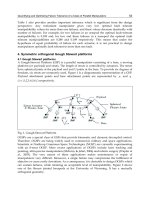
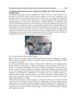
The model of the biped robot SHUR (shown in Fig.1) used in this paper consists of two 6-
DOF legs and a trunk connecting them. Link the sizes and the masses of the links of the
biped are given in Table 1.
name mass
(kg)
Ixx
(kg.m2)
Iyy
(kg.m2)
Izz
(kg.m2)
size
(m)
foot 1.17 0.001248 0.0051309
4
0.0051309 Lf = 0.215
wf = 0.08
hf = 0.08
shin 2.79 0.0381378 0.0381378 0.0018755 Ls = 0.4
thigh 5.94 0.0686441 0.0686441 0.0089843 Lt = 0.36
trunk 40.2 3.13895 2.93628 0.526955 wb =0.22
hb = 0.91
Table 1. Parameter of SHUR model
Fig. 1. Coordinate of a biped robot SHUR
[

]
\
Climbing & Walking Robots, Towards New Applications
92
When the trunk keeps upright and the bottoms of the feet keep horizontal in gait planning,
the posture of the biped robot can be decided by the positions of hip and the ankle of the
swinging leg (Huang, et al, 1999). The center of mass of the robot in x direction
)(tx
hip
plays
an important role in walking stability of forward movement in which the robot tends to fall
down. And
)(tx
hip
is a monotonic increase function similar to the time. So,
)(tx
hip
can be
taken as a reference variable instead of the reference variable, time, which is usually used.
Firstly, the space trajectories of the movements of the hip and the ankle of the swing leg are
programmed with considerations of environmental restrictions on the robot. Then the
relative movements between parts of the biped robot are fixed. Finally, the trajectory of
)(tx
hip
taken time as the reference variable is planed to control the position of ZMP to
realize a stable walking.
The parameters of the bipedal walking in this chapter are set:
The step length of a single step is
0.6
s

Sm=
,
The period of a single step is
0.8
s
Ts=
,
The maximum height the swing leg passing through is
0.2
s
Hm=
.
2.1.1 Spatial path planning for hip
Because of the symmetry and periodicity of the bipedal walking, only the gait of one single
step needs to be planned. Without loss of generality, it is assumed a single-step starts with
the left leg to be in support and the right leg begins to swing.
It is planned that the position of the hip is located at the middle of the gap between the left
foot and right foot at the moment of the support leg switched.
In a single step period,
2
() [ , ], [0, ]
22
s
T
ss
hip
SS
xt whent∈− ∈
(1)
Because of the symmetry and periodicity of the bipedal walking,

hip hip hip hip
() ()zfx zx==
is
a periodic function. The period is
2
s
T
T=
.
When the robot is with single support and the support leg is vertical
() 0
hip
xt=
, the position
of the hip reaches its highest point in whole cycle of bipedal walking:
hip hip shin thigh
(0) max[ ( )]
hip
zzxll==+
(2)
At the moment of the supporting foot switching, the position of the hip reaches its lowest
point in a period for both legs having the geometry constraints. For sure of the satisfaction of
the geometry constraints at the moment of supporting foot switched, it is planned that robot
retains certain flection
0.1h
δ
=
.
Then,
22

hip hip hip shin thigh
() ()min[()] ( )()
22 2
ss s
hip
SS S
zz zxll h
δ
−= = = + − −
(3)
The fluctuation range of the position of the hip in z-direction is:
Non-time Reference Gait Planning and Stability Control for Bipedal Walking
93
22
hip hip shin thigh shin thigh
max[ ( )] min[ ( )] ( ) ( )
2
s
hipmag hip hip
S
zzxzxllll h
δ
=−=+−+−+
(4)
The mid value of the position of the hip is:
hip
1
mid[ ( )] min[ ( )]
2
hip hip hip hipmag

zx zx z=+
(5)
So, we adopt a cosine function:
() cos(2ʌ )[()]
2
hipmag hip
hip hip hip hip
s
zx
zx midzx
S
=× + (6)
The velocity of the hip is:
hipmag
ʌ z
= sin (2ʌ )
2
hip hip hip
hip hip hip
hip s s
zz x
zx x
tx S S
∂∂
==−×
∂∂


(7)
Thus:

( ) 0, ( ) 0, (0) 0
22
ss
hip hip hip
SS
zzz−= = =

(8)
Eq.8 means the trunk has no impact in z-direction at the moment of the supporting foot
switches, which is useful to the smooth change of supporting foot. Substitute the specific
parameters into the functions (Eq.6 and Eq.7), the space path and velocity of hip movement
are as shown in Fig. 2.
Fig. 2. Hip displacement (left) and velocity (right)
2.1.2 Spatial Path in x-direction (
ankle
x
) for the Ankle of the Swing Leg
In order to keep the process of take–off and step down smoothly, the soles of the feet are
planned to be parallel to the ground during the walking process. We set
ankle
x
to be a
function of
hip
x
:
ankle hip ankle hip
() ()
x
fx x x==

(9)
Climbing & Walking Robots, Towards New Applications
94
At the moment of the robot shifting its supporting leg,
() /2
hip s
xt S=±
, the position of
the ankle of the swing leg:
ankle
s
x
S=± .
When the robot stands with one foot vertically, () 0
hip
xt= , the ankle of the swing leg is
just above the ankle of the supported foot ,that is
ankle
0x = .
In order to prevent unwelcome impact during the take-off and step down process, there are
constraints on velocity of the swing leg is:
ankle ankle
() ()0
22
ss
SS
xx−= =

(10)
From above, we use a Sine Function (see Fig.3):

ankle
sin( )
hip
s
s
x
xS
S
π
= (11)
Its speed is:
ankle
ankle hip hip
hip
cos( )
hip
s
x
x
x
xx
xS
ππ
∂
==
∂
 
(12)
Thus:
ankle ankle

() ()0
22
ss
SS
xx−= =

(13)
So this path meets the requirements of no impact during supporting foot switching.
Fig. 3. Ankle displacement (left) and velocity (right) in x-axis of the Swing leg
2.1.3 Spatial Path in z-direction (
ankle
z ) for the Ankle of the Swing Leg
We plan
ankle
z as a function of
hip
x
:
ankle hip ankle hip
() ()zfxzx== (15)
It follows the constraints as:
Constraints for no striking at the moment of take-off and step-down:
Non-time Reference Gait Planning and Stability Control for Bipedal Walking
95
ankle ankle
() ()0
22
ss
SS
zz−= =


(16)
The constraint of space path:
ankle ankle ankle
() ()0,(0)
22
ss
s
SS
zz zH−= = =
(17)
According to the constraints above, we use a trigonometry function (see Fig.4):
hip
ss
ankle
HH
cos(2 )
22
s
x
z
S
π
=+ (18)
The speed of the Ankle is:
hip
s
H
() sin(2 ) ()
ankle

ankle hip hip
hip s s
x
z
zxt xt
xSS
π
π
∂−
==
∂


(19)
Thus
()0, ()0, (0)0
22
ss
ankle ankle ankle
SS
zzz−= = =

(20)
That is, the swing leg will not strike with the ground during take-off and step-down process.
Fig. 4. Ankle displacement (left) and velocity (right) in z-axis of the Swing leg
Synthesize Eq.11 and Eq.18, we can get the spatial path of the ankle of the swing leg (Fig.5):
ankle
hip
ss
ankle

sin( )
HH
cos(2 )
22
hip
s
s
s
x
xS
S
x
z
S
π
π

=
°
°
®
°
=+
°
¯
(21)
In which,
)(tx
hip
is the referenced variable.

Climbing & Walking Robots, Towards New Applications
96
Fig. 5. Spatial path of the ankle of swing leg
2.2 Gait planning based on ZMP stability
Based on periodicity of bipedal walking and the symmetry of left leg and right leg, there are
three equation restraints for
hip
x
:
Position constraints:

(0)
2
s
hip
S
x =−
,
()
2
s
hip s
S
xT=
(22)
Velocity constraint:

(0) ( )
hip hip s
x

xT=

(23)
As well as two inequalities constraints:
In order to save energy as well as to have the unidirectional characteristic of the time, the
speed of the robot’s trunk should be greater than 0.
() 0
hip
xt>

(24)
For sure of bipedal walking is stable,
zmp
x
must be within the support region :
heel zmp toe
x
xx<<
(25)
In order to meet these constraints at the same time, we use quintic polynomial to represent
the trajectory of
hip
x
.

2345
01 2 3 4 5hip
x
aatatatatat=+++++ (26)
Then:

234
12 3 4 5
23
23 4 5
23 4 5
2 6 12 20
hip
hip
x
aatat atat
x a at at at
=+ + + +
=+ + +


(27)
Substituting three constraint equations into Eq.26 and Eq.27, we get three coefficients:
0
(0)
22
s
s
hip
SS
xa=−
 =− (28)
23
234 5
35

() (0) 2
22
hip s hip s s s
x
Tx a aTaT aT=  =− − −

(29)
Non-time Reference Gait Planning and Stability Control for Bipedal Walking
97
23 4
1345
13
() (0)
22
s
hip s hip s s s s
s
S
x
T x S a aT aT aT
T
−= =+ + + (30)
Then we have:
23 4 2
34 5 3 4
32 3 4 5
5345
133
-( )( 2
22 2 2

5
)
2
ss
hip s s s s s
s
s
SS
x
aT aT aT t aT aT
T
aTtatatat
=++ + + +− −
−+++
(31)
23 4 2 3
34 5 3 4 5
234
345
13
()(345)
22
345
s
hip s s s s s s
s
S
x
aT aT aT aT aT aT t
T

at at at
=+ + + +− − −
+++

(32)
Up to now, the question of gait planning have been changed into solving the three
coefficients of the quintic polynomial under the condition of speed inequality restraints
(Eq.24, Eq.25), and maximizing the stability margin of ZMP.
2.3 Gait optimization based on walking stability using GA (Genetic Algorithm)
2.3.1 GA design
Genetic Algorithm (GA) has been known to be robust for search and optimization problems.
GA has been used to solve difficult problems with objective functions that do not posses
properties such as continuity, differentiability, etc. It manipulates a family of possible
solutions that allows the exploration of several promising areas of the solution space at the
same time. GA also makes handling the constraints easy by using a penalty function vector,
which converts a constrained problem to an unconstrained one. In our work, the most
important constraint is the stability, which is verified by the ZMP concept. This paper
applies the GA to design the gait of humanoid robot to obtain maximum stability margin, so
as to enhance the robot’s walking ability.
For application of optimizing using GA, there are four steps:
(1) Decide the variables which need to be optimized and all kinds of constraints;
(2) Decide the coding and decoding method for feasible solution;
(3) Definite a quantified evaluation method to individual adaptability;
(4) Design GA program, determine the operating measure with gene, and set
parameters used in GA.
The parameters are set:
Population scales M=100,
Evolution generations T=1000,
Overlapping probability
c

P=0.7
,
And variation probability
m
P =0.03
The variables to be optimized are:
35
aa a
4
,and
The speed constraint: () 0, [0, ]
hip s
x
ttT>∈

(33)
Climbing & Walking Robots, Towards New Applications
98
2.3.2 The determination of the optimized goal:
Set the projection point of the ankle of the supporting foot as the origin of the coordinate
system (see Fig.1), the length from heel to the origin of the coordinate is
0.08
heel
lm=
, the
length from the toe to the origin of coordinate is
0.135
toe
lm=
,the central position of the

support foot is:
2
toe heel
footcenter
ll
x
−
=
(34)
In a bipedal walking cycle, the ZMP stability in x direction can be expressed as:

heel zmp toe
lxl−< < (35)
The index of
zmp
x
offsetting the center of the support region is:

||
index zmp footcenter
Sxx=−
(36)
The value of the index is smaller, the stable margin is bigger. Therefore the optimizing goal
can be set as:

345
:[(,,)]Object Minimize J a a a
(37)
In which,
345

(, , ) [| () |, [0,]]
zmp footcenter s
Ja a a Max x t x t T=−∈
(38)
Taking the constraints in consideration, the optimizing goal is modified as:
:()Object Minimize J g+
(39)
In which,
00
0
hip
foot hip
x
g
lx
>

=
®
≤
¯


(40)
2.3.3 Optimized results
By using the toolbox of MATLAB Genetic Algorithm for Function Optimization of
Christopher R .Houck, with the optimize process shown in Fig.6 and Fig.7, we get the
optimized values of all variables:

3

5
11.1184
=-13.9498
= 6.9642
a
a
a
4
=
(41)
The value of the optimize goal:
345
( , , ) 0.0555Ja a a = (42)
The minimum distance between X
zmp
and the support region boundary is 0.052 m, so the
stability margin is big enough. Substitute
35
aa a
4
,and
into X
hip
, then the planned gait is
obtained (refer to Fig.8):
Non-time Reference Gait Planning and Stability Control for Bipedal Walking
99
Fig. 6. Average adaptability (left) and the value of the variables (right)
Fig.9 shows that when the position of the center-of-gravity
cg

x
is outside the support region,
the
z
mp
x
of the planning gait optimized by using of Genetic Algorithm is still at the center of
the support region. This optimized gait has greater stability margin, the capacity of anti-
jamming improved during bipedal walking, and the physical feasible of the planned gait is
guaranteed.
Fig. 7. Optimized adaptability
Fig. 8. Optimized Trajectories of X
hip
Climbing & Walking Robots, Towards New Applications
100
Fig. 9. Centre-of-Gravity and ZMP trajectories of the optimized gait
3. Virtual prototype model of humanoid robot
3.1 Mechanical model in ADAMS
For exactly building a virtual prototype of the humanoid robot SHUR, a various
professional soft wares are used. The geometric model of the humanoid robot SHUR is built
in professional three-dimensional CAD soft Pro/E, its dynamics simulation is in ADAMS
soft ware, the design the robot control system is in MATLAB soft ware. Through
ADAMS/Controls interface module, a real-time data channels between MATLAB and
ADAMS is build, and an associated simulation is implemented.
The mechanical system model of the humanoid robot SHUR in ADAMS must include
geometries, constraints, forces, torques and sensors. The procedure of building the model
includes eight steps.
(1) Building part models for all parts of the humanoid robot, then assembly part models
together through applying geometric constraints as the robot being at the posture of
standing.

(2) Setup environment parameters of ADAMS;
(3) Using the interface module of Mechanical/pro between Pro/e and ADAMS, the
assembled model is imported into ADAMS;
(4) Building pairs (joint) between each adjacent links, and applying locomotion
constraint.
(5) Building contact models between feet of the humanoid robot and the ground.
(6) Setting locomotion constraints at particular joints.
(7) Applying driving torques on joints relating to bipedal walking motion.
(8) Building virtual sensors to receive state information of the system
Non-time Reference Gait Planning and Stability Control for Bipedal Walking
101
Fig. 10. Virtual prototype of humanoid robot SHUR
Fig.10 and Fig.11 show the virtual principle prototype of the humanoid robot SHUR,
including 17 movable links, 16 ball hinge joints and the contact models between both feet
and the ground.
Fig. 11. Basic components and main joints of SHUR
Climbing & Walking Robots, Towards New Applications
102
3.2 Virtual prototype system of humanoid robot SHUR
The input and output variables of the model in ADAMS are defined. The input variables are
the required control variables, that is, the driving moment of the joints. The output variable
is the measuring quantity of sensors, which are the state information of the system, mainly
including: angular displacement, angular velocity, and angular acceleration of each joint
and the state of whole robot, such as CoG, ZMP, and inclination state of the robot and so on.
MATLAB soft ware is used to build a control system block diagram of the control system of
humanoid robot SHUR (Fig.12). The ADAMS mechanical system must be included in block
diagram, so as to complete a closed loop system including ADAMS and control system soft
MATLAB.
The simulation of the whole system is processed by using suitable control laws. The 3D solid
models, kinematics, dynamic model and animation simulation of the humanoid robot are

supplied by ADAMS; the expected gait and the control algorithm are supplied by MATLAB,
and the driving moment of each joint is the output of MATLAB. Through the interface
provided by ADAMS/control module, MATLAB provides the control command of the
driving moment of each joint to ADAMS; the latter will feedback the virtual sensor
information of the system states into MATLAB, a real-time closed loop control system is
completed. The result of the simulation may be displayed and saved through data, drawings
and animations in ADAMS.
Fig. 12. Virtual prototype system of the humanoid robot SHUR
4. Non-time reference stability control method
4.1 Principle of stability control through modifying the walking speed
A biped robot may be viewed as a ballistic mechanism that intermittently interacts with its
environment, the ground, through its feet. The supporting foot / ground “joint” is unilateral
for there is no attractive forces, and underactuated since control inputs are absent. Formally,
unilateral and underactuation are the inherent characteristics of biped walking, leading to
the instability problem, especially un-expected falling down around the edge of the support
foot. This stability problem can be measured by ZMP and or be measured by a more visual
index of the degree of inclination of the robot. Almost every humanoid robot has installed
the sensors like gyroscope to measure the degree of inclination of the robot. A virtual
gyroscope is installed on the virtual prototype of the humanoid robot SHUR to measure the
inclination angle of the posture of the upper body. This inclination angle is the object of the
stability control in our research. At the same time, the inclination angle is also used as the
feedback information of the close-loop stability control system.
Expected gait
Controller Humanoid robot
MATLAB
ADAMS
Non-time Reference Gait Planning and Stability Control for Bipedal Walking
103
To simplify the architecture of the controller, a 2-level control structure including
coordination and control levels is introduced (see Fig.13).The coordination level is in charge

of controlling the stability of bipedal walking. The main tasks of coordination level include
gait planning; coordinate the movements of every part and giving command to the control
level. The control levels receive the command from the coordination level and realize the
trajectory tracking controls of every joint of the humanoid robot.
BodyGradient
JointAngle
DrivenTorque
Stability Feedback
Trajectory Feedback
f(u)
Xhip
Function
Body Gradient TimeI ndex
Stability Controller
SHUR
ADAMS Module
DesiredAngle
RealAngle
JointTorque
PID Controllers
Xhip Gait
Non-Time-Reference
GaitPlanner
JointAngle
Scope
BodyGradient
Scope
Fig. 13. Walking control system in MATLAB
The ZMP trajectory can be easily planned to be located in the valid support region at the
phase of off-line gait planning. But in actual walk, there are the differences between the

actual environment and the ideal one, or a modeling error , the impact of foot-ground, as
well as external interference, which cause the real ZMP trajectory differ from the pre-
designed one. If this difference is in open-loop state, the robot walks directly using the
original planned gait, the stability may be broken down, the pre-planned gait can not be
realized, so, it is necessary to correct the gait path on-line.
When people feel about to fell down, they usually quickens the pace to reduce the
overturning moment and gradually restores to stable walk. The changing of instantaneous
velocity can restores the stability
effectively. Restoring the walk stability by changing
instantaneous walk speed nearly has become a person's instinct of responding, which is
gradually gained through the practices of bipedal walking. This paper uses the same
method of human beings to achieve a stable walk. When the robot falls forward or
backward, the strategy lets the robot accelerate or decelerate in the forward locomotion,
then an additional restoring torque reversing the direction of falling will be added on the
robot.
Does not lose the generality, taking robot falling forward around the edge of the toe of the
support foot as an example, this paper uses an on-line correct method to accelerate the
forward locomotion of the robot to restore the walking stability. When the robot is
accelerated forward, there is an additional forward acceleration
0
hip
xΔ>

(43)
The robot receives a backward additional force
0
xhip
FmxΔ=−Δ <

(44)

The backward additional force will produce a restoring moment relating to the support foot,
which is opposite to the direction of falling.
.
yxcmb
MFhΔ=Δ
(45)
In which,
cmb
h
is the height of the center of the mass of the trunk to the ground. The
additional moment
y
MΔ
is helpful for ZMP to restore to the center of the support region.
Climbing & Walking Robots, Towards New Applications
104
For falling forward, this strategy of accelerating forward will also let the swing leg touch the
ground sooner than original planning, so the robot will get a new support, the falling
forward trend will be stopped.
When we off-line planned the robot space path, we had already considered the robot
walking environmental factors like obstacles or the topographic factor like staircase
specification, the ground gradient and so on. Therefore, the online gait modification had
better not to change the robot space path which be planned off-line. Referring to the non-
time gait planning principle, the non-time reference variable is the only one needs to be
modified in the stability control. So the online modify algorithm can be realized easily based
on offline gait planning, and the space path of the robot passing through remains
unchanged.
Applying non-time gait planning algorithm, the whole gait-planning phase is divided into
two phases, (1) planning the space walking path: Taking the forward locomotion of upper-
body as the reference variable, considering the constraint of the environment, the walking

path of a robot without collision with other objects is designed, thus the relating locomotion
of the parts of the robot is obtained; (2) planning the trajectory of the non-time reference
variable: according the constraint of ZMP stability, design the forward locomotion of upper-
body. By changing the forward locomotion of upper-body.
)(tx
hip
, the dynamics
characteristic can be changed to satisfy the walking stability condition while the space
walking path maintains unchanged.
The trajectory of the upper body of the robot in forward direction is:
2345
012345hip
x
aatatatatat=+++++
(46)
Applying non-time reference principle to the trajectory of the upper body in forward
direction, we replace the variable (time t) in the quintic polynomial with a non-time
parameter (time index
index
time
),The time index
index
time
is a function of the time:
()
index
time f t=
. In control and simulation, the time index
index
time

is a discrete time series
basically separated by the sample time interval (in virtual prototype, it is the time step
length of simulation,
SimTimeStep
).
11nn n
index index index
time time SimT imeStep time
++
=+ +Δ
(47)
In which,
index
timeΔ is the time index correction decided according to the stability states of
the robot.
For guarantee the robot will not stop or go back because of the gait correction, the time index
should satisfy:
11nn
index index
time time
++
>
(48)
So the inequality must be satisfied:
index
time SimTimeStepΔ>−
(49)
In certain scope, if
0
index

timeΔ>
, the forward walks speed is accelerated compare to the off-
line planned one, otherwise decelerated. As shown in Fig.14, using a fuzzy controller to
determinate the time index
index
timeΔ
according to the upper body gradient which
corresponding to the states of stability.
Non-time Reference Gait Planning and Stability Control for Bipedal Walking
105
Range (-1,1]
TimeIndex
Range (0,2]
Delta
TimeIndex
1
TimeIndex
Product
Memory
Fuzzy Logic
Controller
du/dt
Derivative
1
Constant1
SimTimeStep
Constant
Add1
Add
1

BodyGradient
Fig. 14. Time index modification system using fuzzy controller
Regarding to general gait planning methods, the planned gaits in joint space are:
() 1,2,
i
f
t i nJoint
θ
== (50)
If we replace the variable t in Eq.50 with the time index
index
time , we can also correct the
gaits online using the non-time reference stability control algorithm, according to the
stability states of the bipedal walking. The relative motion paths of the joints remain
unchanged after the gait correction, which means the robot space motion paths remain
unchanged.
4.2 Design of Fuzzy Controller
Fuzzy control is a combination of fuzzy logic and control technology, and has advantages to
control the systems which are indeterminate, highly nonlinearity and complex. So we adopt
a fuzzy controller to achieve the nonlinearity mapping between the BodyGradient and the
increment of the time index.
A fuzzy controller shown in Fig.16 is built by using the fuzzy controller tool box in
MATLAB. The Inputs of the fuzzy controller are BodyGradient and GradientRate, and the
output is Coefficient. Fig.17 shows the range of values and membership functions of these
input and output variables.
The variable BodyGradient has three ranges: Forward, Okey and Backward.
The variable GradientRate has three ranges: Negative, Neglectable and Positive.
The variable Coefficient is classified into five ranges: Lower, Low, NoChange, Fast, and
Faster.
There are many methods to derive fuzzy rules for the biped control(Pratt, et al,1998), either

from intuitive knowledge of the biped control by human walking demonstration(G.O.A.
Zapata, et al,1999), or information integration(Zhou,2000). Based on intuitive balancing
knowledge, nine fuzzy rules are obtained as shown in Fig.17 (left), and the relationship
between the inputs and the output of the fuzzy controller is shown inFig.17 (right)
Climbing & Walking Robots, Towards New Applications
106
Fig. 15. Structure of the fuzzy system

A. BodyGradient (input) B. Gradient Rate (input)
C. Time exponent modification parameter (output)
Fig. 16. Membership functions of the input and output variables of the fuzzy controller
Non-time Reference Gait Planning and Stability Control for Bipedal Walking
107
Fig. 17. Nine fuzzy rules of the fuzzy controller
Fig. 17. Fuzzy rules (left) and the relationship between the input and output of the controller
(right)
Climbing & Walking Robots, Towards New Applications
108
4.3 Simulations of climbing upstairs
The simulation of climbing up stairs is realized by the virtual prototype of humanoid robot
SHUR, using the non-time reference dynamic stability control strategies. The simulation
parameters include, the height of the stair is 0.15m, and the depth of the stair is 0.2m, the
period of a single step is 0.8s.The beginning and the ending phases of the gait have a single
step period. Fig.18 shows the virtual prototype of the humanoid robot SHUR and the virtual
environment including stairs. Fig.19 shows motion sequences t of climbing upstairs.
5. Conclusions and discussions
A non-time reference gait planning method is proposed. The usual reference variable, time,
is substituted by a non-time variable in gait, so the whole gait-planning phase can be
divided into two phases, (1) planning the space walking path: Taking the forward
locomotion of upper-body as reference variable, considering the constraint of the

environment, the walking path of a robot without collision with other objects is designed,
thus the relative locomotion of the parts of the robot is obtained; (2) planning the trajectory
of the non-time reference variable: according to the constraint of ZMP stability, design the
forward locomotion of upper-body. The gait-planning problem is changed to the
optimization problem. Using the excellent optimization and searching property of Genetic
Algorithm, the gait with good stability is obtained. This non-time reference gait planning
methods has advantages in passing obstacles, climbing upstairs or downstairs and other
similar situation in which the walking path is specified. In the progress of stability control,
the non-time reference variable is the only one need to be modified, so the online modify
algorithm can be realized easily based on offline gait planning.
Combining the non-time reference gait planning method, the intelligent stability control
strategy through modifying the instantaneous walking speed of the robot is proposed.
When the robot falls forward or backward, the strategy lets the robot accelerate or decelerate
in the forward locomotion, then an additional restoring torque reversing the direction of
falling will be added on the robot. For falling forward, this strategy will also let the swing
leg touch the ground sooner than original planning, so the robot will get a new support, the
falling forward trend will be stopped. According to the principle of non-time reference gait
planning, the non-time reference variable is the only one needs to be modified in the
stability control. The incline state of the upper-body, which reflects the stability state of the
robot directly, is used as the input signal of a fuzzy controller; the correction of the non-time
reference trajectory is used as the output of the fuzzy controller. Then the walking speed is
changed, so the gait of the robot is modified online to realize stable dynamic walking
without changing the off-line planned walking space path. For testify the validity of this
strategy, the humanoid robot climbing upstairs is realized using the virtual prototype of
humanoid robot.
Non-time Reference Gait Planning and Stability Control for Bipedal Walking
109
Fig. 18. Virtual prototype of a humanoid robot with virtual environment including stairs
Fig. 19. Motion sequences of a humanoid robot climbing stairs
Climbing & Walking Robots, Towards New Applications

110
6. References
C. Zhou .Neuro-fuzzy gait synthesis with reinforcement learning for a biped walking robot,
Soft Comput. 4 (2000) 238–250.
G.O.A. ;Zapata&R.K.H. Galvao, T. Yoneyama, Extraction fuzzy control rules from
experimental human operator data, IEEE Trans. Systems Man Cybernet. B 29 (1999)
398–406.
Hirai Kazuo; Hirose Masato & Haikawa Yuji(1998). The development of honda humanoid
robot [A]. Proceedings of 1998 IEEE International Conference on Robotics & Automation].
Belgium. May 1998:1321-1326
J.H. Park& K.D. Kim(1998). Biped robot walking using gravity-compensated inverted
pendulum mode and computed torque control, Proc. IEEE Internat. Conf. on Robotics
and Automation, Leuven, Belgium, 1998. vol.4, pp. 3528-3533
J. Pratt & G. Pratt. Intuitive control of a planar bipedal walking robot, in: Proc. of IEEE Conf.
on Robotics and Automation, 1998, pp. 2014–2021.
J. Yamaguchi; N. Kinoshita; A. Takanish, et al(1996). Development of a dynamic biped
walking system for humanoid development of a biped walking robot adapting to
the humans’ living Goor, Proc. IEEE Internat. Conf. on Robotics and Automation,
Minneapolis, MN, 1996, pp. 232–239.
K.Tanie (1999). MITI Humanoid Robotics Project. The 2nd International symposium on
humanoid robot, 1999.Tokyo: 71-76
Q. Li; A. Takanish & I. Kato(1992).Learning control of compensative trunk motion for biped
walking robot based on ZMP stability criterion, Proc. IEEE=RSJ Internat. Workshop
on Intelligent Robotics and Systems, Raleigh, NC, 1992, pp. 597–603.
Q.Huang; H.Arai & K.Tanie(1999). A High Stability Smooth Walking Pattern for Biped
Robot. IEEE International Conference on Robotics and Automation, 1999,pp:65-71
S.Hashimoto, et al (1998).“ Humanoid Robots in Waseda University –Hadaly-2 and
WABIAN” IARP First International Workshop on Humanoid and Human Friendly
Robotics , October Japan , 1998 , pp. I-2: 1-10
S. Kajita& K. Tani(1995)., Experimental study of biped dynamic walking in the linear

inverted pendulum mode, Proc. IEEE Internat. Conf. on Robotics and Automation,
Nagoya, Japan, 1995, pp. 2885–2891.
5
Design Methodology for Biped Robots:
Applications in Robotics and Prosthetics
Máximo Roa, Diego Garzón and Ricardo Ramírez
National University of Colombia
Colombia
1. Introduction
Bipedal walk as an activity requires an excellent sensorial and movement integration to
coordinate the motions of different joints, getting as a result an efficient navigation system
for a changing environment. Main applications of the study of biped walking are in the field
of medical technology, to diagnose gait pathologies, to take surgical decisions, to adequate
prosthesis and orthesis design to supply natural deficiencies in people and for planning
rehabilitation strategies for specific pathologies. The same principles can also be applied to
develop biped machines; in daily situations, a biped robot would be the best configuration
to interact with humans and to get through an environment difficult for navigation. If the
biped robot is designed with human proportions, the robot could manage his way through
spaces designed for humans, like stairs and elevators, and hopefully the interaction with the
robot would be similar to interaction with a human being.
The National University of Colombia has been working on the design and control of biped
robots, supported by two research groups, Biomechanics and Mobile Robots. The joint effort
of the groups has produced three biped robots with successful walks, based on a single idea:
if an appropriate design methodology exists, the resulting hardware must have appropriate
dynamical characteristics, making easier the control of the walking movements. The design
process successfully merges two lines of research in bipedal walk, passive an active walks,
by using gait patterns obtained thanks to the simulation of a kneed passive walker to create
the trajectory followed by the control of an active biped robot. Our actual line of research in
biped robots is to use biped robots reproducing the human gait pattern as engineering tools
to test the behavior of below-knee prostheses, thus producing a biped robot with

heterogeneous legs that allows the evaluation of how the prosthetics influence the normal
gait of the robot while it is walking as a human.
2. Design Methodology
Biped robot design should be based on a design methodology that produces an appropriate
mechanical structure to get the desired walk. We use a design methodology that groups
passive and active walk relying on dynamic models for bipedal gait (Roa et al., 2004). The
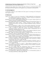
methodology is an iterative process, as shown in Fig. 1. The knowledge of biped robot
O
pen Access Database www.i-techonline.co
m
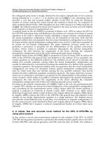
Source: Climbing & Walking Robots, Towards New Applications, Book edited by Houxiang Zhang,
ISBN 978-3-902613-16-5, pp.546, October 2007, Itech Education and Publishing, Vienna, Austria
Climbing & Walking Robots, Towards New Applications
112
dynamics allow us to develop simple and efficient control systems, based on the system
dynamics and not on assumptions of a simplified model, such as the inverted pendulum,
which provides valid results in simulation, but validation is difficult because of the
challenge represented by the measure of position, speed or acceleration of the centre of mass
in a real robotic mechanism.
Change actuator
power
Scale definition
Walking pattern (Passive walking model)
Generation of an initial mechanical design
A
ctuator selection
Estimation of physical characteristics of the robot
Evaluation of dynamic behavior of the robot
(Active walking model)
Construction and control of the robot

Satisfactory behavior
?
NO
Y
ES
Fig. 1. Design methodology for biped robot design
The dynamical model for an actuated walk is the base in the design methodology used here;
it is presented in Section 3. Geometrical and kinematical data are used to solve the model.
Geometric variables of the robot (mass, inertia moment, length, and position of the centre of
mass for each link) can be defined with different criteria, e.g. if the biped robot is intended
to be a model of human gait, it is useful to scale anthropometrical proportions with an
suitable scale factor. These data can be easily acquired using a CAD solid modeler software
for a preliminary design. Kinematical data constitute the gait pattern for the robot. This
pattern can be acquired from two approximations: extracted from a gait analysis of normal
people in a gait laboratory, or generated through the simulation of passive walking models.
The last approach has probed useful to obtain gait patterns at different speeds. The
methodology outlined here assures that the controlled system is mechanically appropriate
to get the desired walking patterns.
3. Dynamical Models for Biped Walkers
The main step in the development of a biped robot is the study and modeling of bipedal
walk. The dynamical study can be accomplished from two points of view: passive and active
walk. In passive walk the main factor is the gravitational influence on artificial mechanisms,
getting a device to walk down a slope without actuators or control. In active walk there are
different actuators which introduce energy to the mechanism so it can walk as desired. The
models, passive and active, begin with a symmetry assumption: the geometric variables for
the two legs are identical. Besides, the two legs are composed of rigid links connected by pin
Design Methodology for Biped Robots: Applications in Robotics and Prosthetics
113
joints, so each joint has just one degree of freedom. Although real walk is a three
dimensional process, the models (and robots) will consider a planar walk, describing the

movements in the sagittal plane (progression plane) of motion.
3.1 Passive Walk
Fig. 2. Kneed-passive walker
McGeer (McGeer, 1990) presented the passive walk concept based on the hypotheses of
understanding human gait as the influence of a neuromotor control mechanism acting on a
device moved only by the gravity influence (Mochon & McMahon, 1980). McGeer first
studied the passive walk through simple models, developed subsequently by different
researchers (Goswami et al., 1996; Garcia et al., 1998). The model used in this work is the
passive dynamic walker with knees (Fig. 2), original of McGeer (McGeer, 1990; Yamakita &
Asano, 2001). The model has three links: stance leg (1), thigh (2) and shank (3), and four
punctual masses (each link has a concentrated mass, and there is one additional mass at the
hip, m
c
). The robot has punctual feet with zero mass. Each link is described with the distal
(a) and proximal (b) lengths to the concentrated mass in the link. The angles lj describe the
angular position of the links with respect to the vertical line, and DŽ is the slope angle.
Fig. 3 shows the diagram of a gait cycle. The cycle begins with both feet on the ground. The
swing leg (thigh and shank) moves freely (under gravity action) until the knee–strike, when
the thigh and shank are aligned and become one single link, preventing a hyperextension in
the knee. This is the beginning of the two-links phase, when the robot behaves as a compass
gait walker. The gait cycle ends when the swinging leg hits the ground (heel-strike); at this
point, the swing and the stance leg interchange their roles, and a new gait cycle begins.
Fig. 3. Gait cycle in kneed-passive walk