Materials Selection and Design (2010) Part 11 doc
Bạn đang xem bản rút gọn của tài liệu. Xem và tải ngay bản đầy đủ của tài liệu tại đây (1.89 MB, 120 trang )
Properties Needed for the Design of
Static Structures
Mahmoud M. Farag, The American University in Cairo
Introduction
ENGINEERING DESIGN can be defined as the creation of a product that satisfies a certain need. A good design should
result in a product that performs its function efficiently and economically within the prevailing legal, social, safety, and
reliability requirements. In order to satisfy such requirements, the design engineer has to take into consideration a large
number of diverse factors:
• Function and consumer requirements,
such as capacity, size, weight, safety, design codes, expected
service life, reliability, maintenance, ease of operation, ease of repair, frequency of failure, initial cost,
operating cost, styling, human factors, noise l
evel, pollution, intended service environment, and
possibility of use after retirement
• Material-related factors,
such as strength, ductility, toughness, stiffness, density, corrosion resistance,
wear resistance, friction coefficient, melting point, therma
l and electrical conductivity, processibility,
possibility of recycling, cost, available stock size, and delivery time
• Manufacturing-related factors,
such as available fabrication processes, accuracy, surface finish, shape,
size, required quantity, delivery time, cost, and required quality
Figure 1 illustrates the relationship among the above three groups. The figure also shows that there are other secondary
relationships between material properties and manufacturing processes, between function and manufacturing processes,
and between function and material properties.
Fig. 1 Factors that should be considered in component design. Source: Ref 1
The relationship between design and material properties is complex because the behavior of the material in the finished
product can be quite different from that of the stock material used in making it. This point is illustrated in Fig. 2, which
shows that in addition to stock material properties, production method and component geometry have direct influence on
the behavior of materials in the finished component. The figure also shows that secondary relationships exist between
geometry and production method, between stock material and production method, and stock material and component
geometry. The effect of component geometry on the behavior of materials is discussed in the following section.
Fig. 2 Factors that should be considered in anticipating the behavior of material in the component. Source:
Ref
1
Reference
1.
M.M. Farag, Selection of Materials and Manufacturing Processes for Engineering Design,
Prentice Hall,
London, 1989
Properties Needed for the Design of Static Structures
Mahmoud M. Farag, The American University in Cairo
Effect of Component Geometry
In almost all cases, engineering components and machine elements have to incorporate design features that introduce
changes in their cross section. For example, shafts must have shoulders to take thrust loads at the bearings and must have
keyways or splines to transmit torques to or from pulleys and gears mounted on them. Under load, such changes cause
localized stresses that are higher than those based on the nominal cross section of the part. The severity of the stress
concentration depends on the geometry of the discontinuity and the nature of the material. A geometric, or theoretical,
stress concentration factor, K
t
, is usually used to relate the maximum stress, S
max
, at the discontinuity to the nominal
stress, S
av
, according to the relationship:
K
t
= S
max
/S
av
(Eq 1)
The value of K
t
depends on the geometry of the part and can be determined from stress concentration charts, such as those
given in Ref 2 and 3. Other methods of estimating K
t
for a certain geometry include photoelasticity, brittle coatings, and
finite element techniques. Table 1 gives some typical values of K
t
.
Table 1 Values of the stress concentration factor K
t
Component shape
Value of critical parameter, K
t
Round shaft with transverse hole
d/D = 0.025 2.65
= 0.05 2.50
= 0.10 2.25
Bending
= 0.20 2.00
d/D = 0.025 3.7
= 0.05 3.6
= 0.10 3.3
Torsion
= 0.20 3.0
Round shaft with shoulder
d/D = 1.5, r/d = 0.05 2.4
r/d = 0.10 1.9
r/d = 0.20 1.55
d/D = 1.1, r/d = 0.05 1.9
= 0.10 1.6
Tension
= 0.20 1.35
d/D = 1.5, r/d = 0.05 2.05
Bending
r/d = 0.10 1.7
r/d = 0.20 1.4
d/D = 1.1, r/d = 0.05 1.9
r/d = 0.10 1.6
r/d = 0.20 1.35
d/D = 1.5, r/d = 0.05 1.7
r/d = 0.10 1.45
r/d = 0.20 1.25
d/D = 1.1, r/d = 0.05 1.25
r/d = 0.10 1.15
Torsion
r/d = 0.20 1.1
Grooved round bar
d/D = 1.1, r/d = 0.05 2.35
r/d = 0.10 2.0
Tension
r/d = 0.20 1.6
d/D = 1.1, r/d = 0.05 2.35
r/d = 0.10 1.9
Bending
r/d = 0.20 1.5
d/D = 1.1, r/d = 0.05 1.65
Torsion
r/d = 0.10 1.4
r/d = 0.20 1.25
Source: Ref 1
Experience shows that, under static loading, K
t
gives an upper limit to the stress concentration value and applies it to
high-strength low-ductility materials. With more ductile materials, local yielding in the very small area of maximum
stress causes some relief in the stress concentration. Generally, the following design guidelines should be observed if the
deleterious effects of stress concentration are to be kept to a minimum:
• Abrupt changes in cross section should be avoided. If they are necessary, generous fillet radii or stress-
relieving grooves should be provided (Fig. 3a).
• Slots and grooves should be provided with generous run-out radii and with fillet radii in all corners (
Fig.
3b).
• Stress-relieving grooves or undercuts should be provided at the end of threads and splines (Fig. 3c).
• Sharp internal corners and external edges should be avoided.
• Oil holes and similar features should be chamfered and the bore should be smooth.
• Weakening features like bolt and oil holes, identific
ation marks, and part numbers should not be located
in highly stressed areas.
• Weakening features should be staggered to avoid the addition of their stress concentration effects (
Fig.
3d).
Fig. 3 Design guidelines for reducing the deleterious effects of stress concentration.
See text for discussion.
Source: Ref 1
References cited in this section
1.
M.M. Farag, Selection of Materials and Manufacturing Processes for Engineering Design,
Prentice Hall,
London, 1989
2.
R.E. Peterson, Stress-Concentration Design Factors, John Wiley and Sons, 1974
3.
J.E. Shigley and L.D. Mitchell, Mechanical Engineering Design, 4th ed., McGraw-Hill, 1983
Properties Needed for the Design of Static Structures
Mahmoud M. Farag, The American University in Cairo
Factor of Safety
The term factor of safety is applied to the factor used in designing a component to ensure that it will satisfactorily perform
its intended function. The main parameters that affect the value of the factor of safety, which is always greater than unity,
can be grouped into:
• Uncertainties associated with material properties due to variations in composition,
heat treatment, and
processing conditions as well as environmental variables such as temperature, time, humidity, and
ambient chemicals. Manufacturing processes also contribute to these uncertainties as a result of
variations in surface roughness, internal stresses, sharp corners, and other stress raisers.
• Uncertainties in loading and service conditions
Generally, ductile materials that are produced in large quantities show fewer property variations than less ductile and
advanced materials that are produced by small batch processes. Parts manufactured by casting, forging, and cold forming
are known to have variations in properties from point to point.
To account for uncertainties in material properties, the factor of safety is used to divide into the nominal strength (S) of
the material to obtain the allowable stress (S
a
) as follows:
S
a
= S/n
s
(Eq 2)
where n
s
is the material factor of safety.
In simple components, S
a
in the above equation can be viewed as the minimum allowable strength of the material.
However there is some danger involved in this use, especially in the cases where the load-carrying capacity of a
component is not directly related to the strength of the material used in making it. Examples include long compression
members, which could fail as a result of buckling, and components of complex shapes, which could fail as a result of
stress concentration. Under such conditions it is better to consider S
a
as the load-carrying capacity that is a function of
both material properties and geometry of the component.
In assessing the uncertainties in loading, two types of service conditions have to be considered:
• Normal working conditions, which the component has to endure during its intended service life
• Limited working conditions, such as overload
ing, which the component is only intended to endure on
exceptional occasions, and which if repeated frequently could cause premature failure of the component
In a mechanically loaded component, the stress levels corresponding to both normal and limited working conditions can
be determined from a duty cycle. The normal duty cycle for an airframe, for example, includes towing and ground
handling, engine run, take-off, climb, normal gust loadings at different altitudes, kinetic and solar heating, descent, and
normal landing. Limited conditions can be encountered in abnormally high gust loadings or emergency landings.
Analyses of the different loading conditions in the duty cycle lead to determination of the maximum load that will act on
the component. This maximum load can be used to determine the maximum stress, or damaging stress, which if exceeded
would render the component unfit for service before the end of its normal expected life. The load factor of safety (n
l
) in
this case can be taken as:
n
l
= P/P
a
(Eq 3)
where P is the maximum load and P
a
is normal load.
The total or overall factor of safety (n) that combines the uncertainties in material properties and external loading
conditions can be calculated as:
n = n
s
· n
l
(Eq 4)
Factors of safety ranging from 1.1 to 20 are known, but common values range from 1.5 to 10.
In some applications a designer is required to follow established codes when designing certain components, for example,
pressure vessels, piping systems, and so forth. Under these conditions, the factors of safety used by the writers of the
codes may not be specifically stated, but an allowable working stress is given instead.
Properties Needed for the Design of Static Structures
Mahmoud M. Farag, The American University in Cairo
Probability of Failure
As discussed earlier, the actual strength of the material in a component could vary from one point to another and from one
component to another. In addition, it is usually difficult to precisely predict the external loads acting on the component
under actual service conditions. To account for these variations and uncertainties, both the load-carrying capacity S and
the externally applied load P can be expressed in statistical terms. As both S and P depend on many independent factors,
it would be reasonable to assume that they can be described by normal distribution curves. Consider that the load-carrying
capacity of the population of components has an average of and a standard deviation
S
while the externally applied
load has an average of and a standard deviation
P
. The relationship between the two distribution curves is important
in determining the factor of safety and reliability of a given design. Figure 4 shows that failure takes place in all the
components that fall in the area of overlap of the two curves, that is, when the load-carrying capacity is less than the
external load. This is described by the negative part of the (S - P) curve of Fig. 4. Transforming the distribution ( - )
to the standard normal deviate z, the following equation is obtained:
z = [(S - P) - ( - )]/[(
S
)
2
+ (
P
)
2
]
1/2
(Eq 5)
From Fig. 4, the value of z at which failure occurs is:
z = - (S - P)/[(
S
)
2
+ (
P
)
2
]
1/2
(Eq 6)
Fig. 4 Effect of variations in load and strength on the failure of components. Source: Ref 1
For a given reliability, or allowable probability of failure, the value of z can be determined from cumulative distribution
function for the standard normal distribution. Table 2 gives some selected values of z that will result in different values of
probabilities of failure.
Table 2 Values of z and corresponding levels of reliability and probability of failure
z Reliability
Probability of
failure
-1.00
0.8413 0.1587
-1.28
0.9000 0.1000
-2.33
0.9900 0.0100
-3.09
0.9990 0.0010
-3.72
0.9999 0.0001
-4.26
0.99999 0.00001
-4.75
0.999999 0.000001
Knowing
S
,
P
, and the expected , the value of can be determined for a given reliability level. As defined earlier,
the factor of safety in the present case is simply S/P. The following example illustrates the use of the above concepts in
design; additional discussion of statistical methods is provided in the article "Statistical Aspects of Design" in this
Volume.
Example 1: Estimating Probability of Failure.
A structural element is made of a material with an average tensile strength of 2100 MPa. The element is subjected to a
static tensile stress of an average value of 1600 MPa. If the variations in material quality and load cause the strength and
stress to vary according to normal distributions with standard deviations of
S
= 400 and
P
= 300, respectively, what is
the probability of failure of the structural element? The solution can be derived as follows: From Fig. 4, ( - ) = 2100 -
1600 = 500 MPa, standard deviation of the curve ( - ) = [(400)
2
+ (300)
2
]
1/2
= 500; from Eq 6, z = -500/500 = -1.
Thus, from Table 2, the probability of failure of the structural element is 0.1587 (15.87%), which is too high for many
practical applications.
One solution to reduce the probability of failure is to impose better quality measures on the production of the material and
thus reduce the standard deviation of the strength. Another solution is to increase the cross-sectional area of the element
in order to reduce the stress. For example, if the standard deviation of the strength is reduced to
S
= 200, the standard
deviation of the curve ( - ) will be [(200)
2
+ (300)
2
]
1/2
= 360, z = -500/360 = -1.4, which, according to Table 2, gives
a more acceptable probability of failure value of 0.08 (8%).
Alternatively, if the average stress is reduced to 1400 MPa, ( - ) = 700 MPa, z = -700/500 = -1.4, with a similar
probability of failure as the first solution.
Experimental Methods. As the above discussion shows, statistical analysis allows the generation of data on the
probability of failure and reliability, which is not possible when a deterministic safety factor is used. One of the
difficulties with this statistical approach, however, is that material properties are not usually available as statistical
quantities. In such cases, the following approximate method can be used.
In the case where the experimental data are obtained from a reasonably large number of samples, more than 100, it is
possible to estimate statistical data from nonstatistical sources that only give ranges or tolerance limits. In this case, the
standard deviation
S
is approximately given by:
S
= (maximum value of property
- minimum value)/6
(Eq 7)
This procedure is based on the assumption that the given limits are bounded between plus and minus three standard
deviations.
If the results are obtained from a sample of about 25 tests, it may be better to divide by 4 in Eq 7 instead of 6. With a
sample of about 5, it is better to divide by 2.
In the cases where only the average value of strength is given, the following values of coefficient of variation, which is
defined as ' =
S
/S can be taken as typical for metallic materials: ' = 0.05 for ultimate tensile strength, and ' = 0.07
for yield strength.
Reference cited in this section
1.
M.M. Farag, Selection of Materials and Manufacturing Processes for Engineering Design,
Prentice Hall,
London, 1989
Properties Needed for the Design of Static Structures
Mahmoud M. Farag, The American University in Cairo
Designing for Static Strength
The design and materials selection of a component or structure under static loading can be based on static strength and/or
stiffness depending on the service conditions and the intended function.
In the case of ductile materials, designs based on the static strength usually aim at avoiding yielding of the component.
The manner in which the yield strength of the material affects the design depends on the loading conditions and type of
component, as illustrated in the following cases.
Designing for Axial Loading. When the component is subjected to uniaxial stress, yielding takes place when the local
stress reaches the yield strength of the material. The critical cross-sectional area, A, of such a component can be estimated
as:
A = K
t
n P/YS
(Eq 8)
where K
t
is the stress concentration factor (described in the section "Effect of Component Geometry" in this article), P is
the applied load, n is the factor of safety, (described in the section "Factor of Safety" in this article), and YS is the yield
strength of the material.
Designing for Torsional Loading. The critical cross-sectional area of a circular shaft subjected to torsional loading
can be determined from the relationship:
2 I
p
/d = K
t
n T/
max
(Eq 9)
where d is the shaft diameter at the critical cross section,
max
is the shear strength of the material, T is the transmitted
torque, and I
p
is the polar moment of inertia of the cross section. (I
p
= d
4
/32 for a solid circular shaft; I
p
= ( -
)/32 for a hollow circular shaft of inner diameter d
i
and outer diameter d
o
.)
While Eq 9 gives a single value for the diameter of a solid shaft, a large combination of inner and outer diameters can
satisfy the relationship in the case of a hollow shaft. Under such conditions, either one of the diameters or the required
thickness has to be specified in order to calculate the other dimension.
The ASTM code of recommended practice for transmission shafting gives an allowable value of shear stress of 0.3 of the
yield or 0.18 of the ultimate tensile strength, whichever is smaller. With shafts containing keyways, ASTM recommends a
reduction of 25% of the allowable shear strength to compensate for stress concentration and reduction in cross-sectional
area.
Designing for Bending. When a relatively long beam is subjected to bending, the bending moment, the maximum
allowable stress, and dimensions of the cross section are related by:
Z = (n M)/YS
(Eq 10)
where M is the bending moment and Z is the section modulus (Z = I/c, where I is the moment of inertia of the cross
section with respect to the neutral axis normal to the direction of the load, and c is the distance from center of gravity of
the cross section to the outermost fiber). Bending moment can be determined by consulting a standard reference on the
strength of materials, such as Ref 4.
Reference cited in this section
4.
W.C. Young, Roark's Formulas for Stress and Strain, 6th ed., McGraw-Hill, 1989
Properties Needed for the Design of Static Structures
Mahmoud M. Farag, The American University in Cairo
Designing for Stiffness
In addition to being strong enough to resist the expected service loads, there may also be the added requirement of
stiffness to ensure that deflections do not exceed certain limits. Stiffness is important in applications such as machine
elements to avoid misalignment and to maintain dimensional accuracy of machine parts.
Design of Beams. The deflection of a beam under load can be taken as a measure of its stiffness, and this depends on
the position of the load, the type of beam, and the type of supports. For example, a beam that is simply supported at both
ends suffers maximum deflection (y) in its middle when subjected to a concentrated central load (P). In this case the
maximum deflection, y, is a function of both E and I, as follows:
y = (P · L
3
) / (48 · E · I)
(Eq 11)
where L is the length of the beam, E is Young's modulus of the beam material, and I is the second moment of area of the
beam cross section with respect to the neutral axis.
Design of Columns. Columns and struts, which are long slender parts, are subject to failure by elastic instability, or
buckling, if the applied axial compressive load exceeds a certain critical value, P
cr
. The Euler column formula is usually
used to calculate the value of P
cr
, which is a function of the material, geometry of the column, and restraint at the ends.
For the fundamental case of a pin-ended column, that is, ends are free to rotate around frictionless pins, P
cr
is given as:
P
cr
=
2
E I/L
2
(Eq 12)
where I is the least moment of inertia of the cross-sectional area of the column, and L is the length of the column.
The above equation can be modified to allow for end conditions other than the pinned ends. The value of P
cr
for a column
with both ends fixed built-in as part of the structure is four times the value given by Eq 12. On the other hand, the
critical load for a free-standing column one end is fixed and the other free as in a cantilever P
cr
is only one-quarter of
the value given by Eq 12.
The Euler column formula given above shows that the critical load for a given column is only a function of E and I and is
independent of the compressive strength of the material. This means that resistance to buckling of a column of a given
material and a given cross-sectional area can be increased by distributing the material as far as possible from the principal
axes of the cross section to increase I. Hence, tubular sections are preferable to solid sections. Reducing the wall thickness
of such sections and increasing the transverse dimensions increases the stability of the column. However, there is a lower
limit for the wall thickness below which the wall itself becomes unstable and causes local buckling.
Experience shows that the values of P
cr
calculated according to Eq 12 are higher than the buckling loads observed in
practice. The discrepancy is usually attributed to manufacturing imperfections, such as lack of straightness of the column
and lack of alignment between the direction of the compressive load and the axis of the column. This discrepancy can be
accounted for by using an appropriate imperfection parameter or a factor of safety. For normal structural work, a factor of
safety of 2.5 is usually used. As the extent of the above imperfections is expected to increase with increasing slenderness
of the column, it is suggested that the factor of safety be increased accordingly. A factor of safety of 3.5 is recommended
for columns with [L(A/I)
1/2
] > 100, where A is cross-sectional area.
Equation 12 shows that the value of P
cr
increases rapidly as the length of the column, L, decreases. For a short enough
column, P
cr
becomes equal to the load required for yielding or crushing of the material in simple compression. Such a
case represents the limit of applicability of the Euler formula as failure takes place by yielding or fracture rather than
elastic instability. Such short columns are designed according to the procedure described for simple axial loading.
Design of Shafts. The torsional rigidity of a component is usually measured by the angle of twist, , per unit length.
For a circular shaft, is given in radians by:
= T/G I
p
(Eq 13)
where G is the modulus of elasticity in shear, and:
G = E/[2(1 + )]
(Eq 14)
where is Poisson's ratio.
The usual practice is to limit the angular deflection in shafts to about 1° ( /180 radians) in a length of 20 times the
diameter.
Properties Needed for the Design of Static Structures
Mahmoud M. Farag, The American University in Cairo
Selection of Materials for Static Strength
Static Strength and Isotropy. The resistance to static loading is usually measured in terms of yield strength,
ultimate tensile strength, and compressive strength. When the material does not exhibit a well-defined yield point, the
stress required to cause 0.1 or 0.2% plastic strain, the proof stress, is used instead. (This is usually called the 0.2% offset
yield strength.) For most ductile wrought metallic materials, the tensile and compressive strengths are very close, and in
most cases only the tensile strength is given. However, brittle materials like gray cast iron and ceramics are generally
stronger in compression than in tension. In such cases, both properties are usually given. For polymeric materials, which
usually do not have a linear stress-strain curve, and whose static properties are very temperature dependent, other design
methods must be used; additional information is provided in the article "Design with Plastics" in this Volume.
Although many engineering materials are almost isotropic, there are important cases where significant anisotropy exists.
In the latter case, the strength depends on the direction in which it is measured. The degree of anisotropy depends on the
nature of the material and its manufacturing history. Anisotropy in wrought metallic materials is more pronounced when
they contain elongated inclusions and when processing consists of repeated deformation in the same direction.
Composites reinforced with unidirectional fibers also exhibit pronounced anisotropy. Anisotropy can be useful if the
principal external stress acts along the direction of highest strength.
The level of strength in engineering materials may be viewed either in absolute terms or relative to similar materials.
For example, it is generally understood that high-strength steels have tensile strength values in excess of 1400 MPa (200
ksi), which is also high strength in absolute terms. Relative to light alloys, however, an aluminum alloy with a strength of
500 MPa (72 ksi) would also be designated a high-strength alloy even though this level of strength is low for steels.
From the design point of view, it is more convenient to consider the strength of materials in absolute terms. From the
materials and manufacturing point of view, however, it is important to consider the strength as an indication of the degree
of development of the material concerned, that is, relative to similar materials. This is because highly developed materials
are often complex, more difficult to process, and relatively more expensive. Figure 5 gives the strength of some materials
both in absolute terms and relative to similar materials. In a given group of materials, the medium-strength members are
usually more widely used because they generally combine optimal strength, ease of manufacture, and economy. The
most-developed members in a given group of materials are usually highly specialized, and as a result they are produced in
much lower quantities. The low-strength members of a given group are usually used to meet requirements other than
strength. For example, electrical and thermal conductivities, formability, or corrosion resistance may be more important
than strength in some applications.
Fig. 5 Comparison of various engineering materials on the basis of tensile strength. Source: Ref 1
Frequently, higher-strength members of a given group of materials are more expensive. However, using a stronger but
more expensive material could result in a reduction of the total cost of the finished component. This is because less
material would be used, and consequently processing cost could also be less.
Weight and Space Limitations. The load-carrying capacity of a given component is a function of both the strength
of the material used in making it and its geometry and dimensions. This means that a lower-strength material can be used
in making a component to bear a certain load, provided that its cross-sectional area is increased proportionally. However,
the designer is not usually completely free in choosing the strength level of the material selected for a given part. Other
factors such as space and weight limitations could limit the choice.
Weight limitations are encountered with many applications including aerospace, transport, construction, and portable
appliances. In such cases, the strength/density, or specific strength, becomes an important basis for comparing the
different materials. Figure 6 compares the materials of Fig. 5 on the basis of specific strength, which is the tensile strength
of a material divided by its density. The figure shows a clear advantage of the fiber-reinforced composites over other
materials.
Fig. 6 Comparison of various engineering materials on the basis of specific tensile strength. Source: Ref 1
Using stronger material will allow smaller cross-sectional area and smaller total volume of the component. It should be
noted, however, that reducing the cross-sectional area below a certain limit could cause failure by buckling due to
increased slenderness of the part.
Example 2: Materials Selection for a Cylindrical Compression Element.
A load of 50 kN is to be supported on a cylindrical compression element of 200 mm length. As the compression element
has to fit with other parts of the structure, its diameter should not exceed 20 mm. Weight limitations are such that the
mass of the element should not exceed 0.25 kg. Table 3 shows the calculated diameter of the compression element when
made of different materials. The diameter is calculated on the basis of strength and on the basis of buckling. The larger
value for a given material is used to calculate the mass of the element. The results in Table 3 show that only epoxy-62%
Kevlar satisfies both the diameter and weight limits for the compression element.
Table 3 Comparison of materials considered for a cylindrical compression element
See Example 2 in text.
Material Strength,
MPa
Elastic
modulus,
GPa
Specific
gravity
Diameter
based on
strength,
mm
Diameter
based on
buckling,
mm
Mass
based on
larger diam,
kg
Remarks
Steels
ASTM A 675, grade 45
155 211 7.8 20.3 15.75 . . . Reject
(a)
ASTM A 675, grade 80
275 211 7.8 15.2 15.75 0.3 Reject
(b)
ASTM A 715, grade 80
550 211 7.8 10.8 15.75 0.3 Reject
(b)
Aluminum
2014-T6
420 70.8 2.7 12.3 20.7 . . . Reject
(a)
Plastics and composites
Nylon 6/6
84 3.3 1.14 27.5 44.6 . . . Reject
(a)
Epoxy-70% glass
2100 62.3 2.11 5.5 21.4 . . . Reject
(a)
Epoxy-62% Kevlar
1311 82.8 1.38 7.0 19.9 0.086 Accepted
Source: Ref 1
(a)
Material is rejected because it violates the limits on diameter.
(b)
Material is rejected because it violates the limits on weight.
Reference cited in this section
1.
M.M. Farag, Selection of Materials and Manufacturing Processes for Engineering Design, Prentice H
all,
London, 1989
Properties Needed for the Design of Static Structures
Mahmoud M. Farag, The American University in Cairo
Selection of Materials for Stiffness
Deflection under Load. As discussed in the section "Design of Beams" in this article, the stiffness of a component
may be increased by increasing its second moment of area, which is computed from the cross-sectional dimensions,
and/or by selecting a high-modulus material for its manufacture.
An important characteristic of metallic materials is that their elastic moduli are very difficult to change by changing the
composition or heat treatment. Using high-strength materials in attempts to reduce weight usually comes at the expense of
reduced cross-sectional area and reduced second moment of area. This could adversely affect stiffness of the component
if the elastic constant of the new strong material does not compensate for the reduced second moment of area.
Selecting materials with higher elastic constant and efficient disposition of material in the cross section are essential in
designing beams for stiffness. Placing material as far as possible from the neutral axis of bending is generally an effective
means of increasing I for a given area of cross section. See the discussion of shape factor in the article "Performance
Indices" in this Volume.
When designing with plastics, whose elastic modulus is 10 to 100 times less than that of metals, stiffness must be given
special consideration. This drawback can usually be overcome by making some design adjustments. These usually include
increasing the second moment of area of the critical cross section, as shown in the following example.
Example 3: Design Changes Required for Materials Substitution.
This example considers the design changes required when substituting high-density polyethylene (HDPE) for stainless
steel in making a fork for a picnic set while maintaining similar stiffness. The narrowest cross section of the original
stainless steel fork is rectangular with an area of 0.6 by 5 mm.
Analysis:
• E for stainless steel = 210 GPa.
• E for HDPE = 1.1 GPa.
• I for the stainless steel section = 5 × (0.6)
3
/12 = 0.09 mm
4
.
• From Eq 11, EI should be kept constant for equal deflection under load.
• EI for stainless steel = 210 × 0.09 = 18.9.
• EI for HDPE design = 1.1 × I.
• I for HDPE design = 17.2 mm
4
. Taking a channel section of thickness 0.5 mm, web height 4 mm, a
nd
width 8 mm, I = [8 × (4)
3
- 7 × (3.5)
3
]/12 = 17.7 mm
4
, which meets the required value.
• Area of the stainless steel section = 3 mm
2
.
• Area of the HDPE section = 7.5 mm
2
.
• The specific gravity of stainless steel is 7.8 and that of HDPE is 0.96.
• Relative weight of HDPE/stainless steel = (7.5 × 0.96)/(3 × 7.8) = 0.3.
Weight Limitations. In applications where both the stiffness and weight of a structure are important, it becomes
necessary to consider the stiffness/weight (specific stiffness), of the structure. In the simple case of a structural member
under tensile or compressive load, the specific stiffness is given by E/ , where is the density of the material. In such
cases, the weight of a member of a given stiffness can be easily shown to be proportional to /E and can be reduced by
selecting a material with lower density or higher elastic modulus. When the component is subjected to bending, the
dependence of the weight on and E is not as simple. From Eq 11 it can be shown that the weight w of a simply
supported beam of square cross-sectional area is given by:
(Eq 15)
Related information is provided in the article "Performance Indices" in this Volume.
Equation 15 shows that for a given deflection y under load P, the weight of the beam is proportional to ( /E
1/2
). As E in
this case is present as the square root, it is not as effective as in controlling the weight of the beam. It can be similarly
shown that the weight of the beam in the case of a rectangular cross section is proportional to ( /E
1/3
), which is even less
sensitive to variations in E. This change in the effectiveness of E in affecting the specific stiffness of structures as the
mode of loading and shape change, is shown in Table 4.
Table 4 Comparison of the stiffness of selected engineering materials
Material Modulus of
elasticity
(E), GPa
Density ( ),
mg/m
3
E/
× 10
-5
E
1/2
/
× 10
-2
E
1/3
/
Steel (carbon and low alloy)
207 7.825 26.5 5.8 35.1
Aluminum alloys (average)
71 2.7 26.3 9.9 71.2
Magnesium alloys (average)
40 1.8 22.2 11.1 88.2
Titanium alloys (average)
120 4.5 26.7 7.7 50.9
Epoxy-73% E-glass fibers
55.9 2.17 25.8 10.9 81.8
Epoxy-70% S-glass fibers
62.3 2.11 29.5 11.8 87.2
Epoxy-63% carbon fibers
158.7 1.61 98.6 24.7 156.1
Epoxy-62% aramid fibers
82.8 1.38 60 20.6 146.6
Source: Ref 1
Buckling Strength. Another selection criterion that is also related to the elastic modulus of the material and cross-
sectional dimensions is buckling under compressive loading. The compressive load, P
b
, that can cause buckling of a strut
is given by Euler formula (Eq 12).
Equation 12 shows that increasing E and I will increase the load-carrying capacity of the strut. For an axially symmetric
cross section, the weight of a strut, w, is given by:
(Eq 16)
Equation 16 shows that the weight of an axisymmetric strut can be reduced by reducing or by increasing E of the
material, or both. However, reducing is more effective, as E is present as the square root. In the case of a panel
subjected to buckling, it can be shown that the weight is proportional to ( /E
1/3
).
Reference cited in this section
1.
M.M. Farag, Selection of Materials and Manufacturing Processes for Engineering Design,
Prentice Hall,
London, 1989
Properties Needed for the Design of Static Structures
Mahmoud M. Farag, The American University in Cairo
Types of Mechanical Failure under Static Loading at Normal Temperatures
Generally, a component can be considered to have failed when it does not perform its intended function with the required
efficiency. The general types of mechanical failure encountered in practice are:
• Yielding of the component material under static loading.
Yielding causes permanent deformation that
could result in misalignment or hindrance to mechanical movement.
• Buckling.
This type of failure takes place in slender columns when they are subjected to compressive
loading, or in thin-walled tubes when subjected to torsional loading.
• Failure by fracture due to static overload. This type of failure can be cons
idered an advanced stage of
failure by yielding. Fracture can be either ductile or brittle.
• Failure due to the combined effect of stresses and corrosion.
This usually takes place by fracture due to
cracks at stress concentration points, for example, caustic cracking around rivet holes in boilers.
Of the above types of mechanical failure, the first two do not usually involve actual fracture, and the component is
considered to have failed when its performance is below acceptable levels. On the other hand, the latter two types involve
actual fracture of the component, and this could lead to unplanned load transfer to other components and perhaps other
failures.
Properties Needed for the Design of Static Structures
Mahmoud M. Farag, The American University in Cairo
Causes of Failure of Engineering Components
As discussed earlier, the behavior of a material in service is governed not only by its inherent properties, but also by the
stress system acting on it and the environment in which it is operating. Causes of failure of engineering components can
be classified into the following main categories:
• Design deficiencies.
Failure to evaluate working conditions correctly due to the lack of reliable
information on loads and service conditions is a major cause of i
nadequate design. Incorrect stress
analysis, especially near notches, and complex changes in shape could also be a contributing factor.
• Poor selection of materials.
Failure to identify clearly the functional requirements of a component could
lead to the s
election of a material that only partially satisfies these requirements. As an example, a
material can have adequate strength to support the mechanical loads, but its corrosion resistance is
insufficient for the application.
• Manufacturing defects. Incorre
ct manufacturing could lead to the degradation of an otherwise
satisfactory material. Examples are decarburization and internal stresses in a heat-
treated component.
Poor surface finish, burrs, identification marks, and deep scratches due to mishandling co
uld lead to
failure under fatigue loading.
• Exceeding design limits and overloading.
If the load, temperature, speed, and so forth, are increased
beyond the limits allowed by the factor of safety in design, the component is likely to fail. Subjecting
the e
quipment to environmental conditions for which it was not designed also falls under this category.
An example here is using a freshwater pump for pumping seawater.
• Inadequate maintenance and repair. When maintenance schedules are ignored and repairs are p
oorly
carried out, service life is expected to be shorter than anticipated in the design.
As this article has described, various material properties influence the design of components. The type of property and the
sensitivity of the design to variations in this property depend on the component geometry and type of load.
Underestimation of the load and/or overestimation of the material property and service conditions could lead to failure in
service.
Properties Needed for the Design of Static Structures
Mahmoud M. Farag, The American University in Cairo
References
1. M.M. Farag, Selection of Materials and Manufacturing Processes for Engineering Design,
Prentice Hall,
London, 1989
2. R.E. Peterson, Stress-Concentration Design Factors, John Wiley and Sons, 1974
3. J.E. Shigley and L.D. Mitchell, Mechanical Engineering Design, 4th ed., McGraw-Hill, 1983
4. W.C. Young, Roark's Formulas for Stress and Strain, 6th ed., McGraw-Hill, 1989
Properties Needed for the Design of Static Structures
Mahmoud M. Farag, The American University in Cairo
Selected References
• V.J. Colangelo and F.A. Heiser, Analysis of Metallurgical Failures, John Wiley and Sons, 1987
• N.H. Cook, Mechanics and Materials for Design, McGraw-Hill, 1985
• F.A.A. Crane and J.A. Charles, Selection and Use of Engineering Materials, Butterworths, 1984
• M.M. Farag, Materials Selection for Engineering Design, Prentice Hall, London, 1997
Design for Fatigue Resistance
Erhard Krempl, Rensselaer Polytechnic Institute
Introduction
FATIGUE is a gradual process caused by repeated application of loads, such that each application of stress causes some
degradation or damage of the material or component. An appropriate measure of deterioration or damage has not been
found, and this fact makes fatigue design difficult.
The design of components against fatigue failure may involve several considerations of irregular loading, variable
temperature, and environment. In this article, the effect of environment is excluded. The effects of environment on
material performance are considered elsewhere in this Volume.
The main objective here is the discussion of design considerations against fatigue related to material performance under
mechanical loading at constant temperature (isothermal fatigue, or simply fatigue). In this article, periodic loading of
specimens is considered, and the material properties related to fatigue derived from these tests are discussed.
Design methods considering the irregular nature of actual load applications, which requires the statistical treatment of the
load histories and their translation into load spectra, cycle counting methods, and damage accumulation will not be
discussed. These topics are addressed in more detail in Fatigue and Fracture, Volume 19 of ASM Handbook (Ref 1).
This article reviews "traditional" methods of fatigue design. In recent years, the fracture mechanics approach to crack
propagation has gained acceptance in the prediction of fatigue life. In this approach, crack initiation is neglected and
crack propagation to final failure is considered. This method can give a conservative estimate of fatigue life. There has
been considerable success with this method. However, the treatment of short cracks, the propagation of cracks for
negative R-ratios, and for irregular loading, crack closure effects and multiaxial loadings provide significant challenges.
Reference 2 gives an introduction to the current research in this area.
In addition, the design methods reviewed in this article focus principally on smooth and notched components.
Mechanically fastened joints and welded joints require special attention. In particular, such joints tend to negate alloy and
composition effects. More detailed information on fatigue of welds and mechanical joints is contained in Ref 1, 3, and 4.
References
1.
Fatigue and Fracture, Vol 19, ASM Handbook, ASM International, 1996
2.
M.R. Mitchell and R.W. Landgraf, Ed., Advances in Fatigue Lifetime Predictive Techniques,
STP 1122,
ASTM, 1992
3.
H.O. Fuchs and R.I. Stephens, Metal Fatigue in Engineering, John Wiley & Sons, 1980
4.
M.L. Sharp and G.E. Nordmark, Fatigue Design of Aluminum Components and Structures, McGraw-
Hill,
1996
Design for Fatigue Resistance
Erhard Krempl, Rensselaer Polytechnic Institute
The Fatigue Process
The fatigue process consists of a crack initiation and a crack propagation phase. The demarcation between these two
phases is, however, not clearly defined. There is no general agreement when (or at what crack size) the crack initiation
process ends, and the crack growth process begins. Nonetheless, the separation of the fatigue process in initiation and
propagation phases has been developing during the last forty years. The tendency is now to investigate crack growth of
preexisting flaws and to neglect the crack initiation process. This method has been driven by the development of the
fracture mechanics approach. Previously, the cycles-to-failure needed to completely separate the test specimens were
reported, and no separation in crack initiation and crack growth life had been made.
For metals and alloys, two regimes of the fatigue phenomenon are generally considered high-cycle fatigue and low-cycle
fatigue.
High-cycle fatigue involves nominally linear elastic behavior and causes failure after more than approximately 100,000
cycles. As the loading amplitude is decreased, the cycles-to-failure increase. For many alloys, a fatigue (endurance) limit
exists beyond 10
6
cycles. The endurance or fatigue limit represents a stress level below which fatigue life appears to be
infinite upon extrapolation. However, fatigue limits from controlled laboratory tests (often limited from 10
6
to 10
8
cycles)
are not necessarily valid in application environments. For example, a fatigue limit can be eradicated by one large overload
or the onset of additional crack-initiation mechanisms such as corrosion at the surface. Moreover, even though testing
ceases at 10
6
or 10
8
cycles for practical reasons, it is known that fatigue limits cannot be extrapolated to infinity. In some
cases, there may be a change in failure mechanisms at lives above 10
6
or 10
8
cycles.
Due to the nominally elastic behavior, dissipation is small and high-frequency testing at small amplitudes can be
performed without causing self-heating of the specimen. In mechanical testing machines, frequencies up to 300 Hz are
possible. Usual testing speeds, however, are below 100 Hz. At this frequency, approximately 8.6 × 10
6
cycles are
accumulated per day. To impose 8.6 × 10
8
cycles, more than a hundred days of testing time at 100 Hz are required. It is
therefore no surprise that fatigue data extending to more than 10
8
cycles are hard to find.
Stresses involving inelastic deformation so that a significant stress-strain hysteresis loop develops during cyclic loading
lead to low-cycle fatigue failure, usually in less than 100,000 cycles. Cyclic inelastic deformation causes dissipation of
energy, which can lead to significant self-heating of a specimen if a high frequency is used for testing. This is one reason
why low-cycle fatigue testing is usually performed at frequencies below 1 Hz. Low-cycle fatigue investigations started in
the 1950s in response to failures that were found in power-generation equipment. The problems were caused by frequent
start/stop operations and thermal stresses induced by temperature changes.
The simultaneous advent of servocontrolled testing machines, using feedback control, clip-on extensometers, and
computer control made testing relevant to the engineering problem at hand and established low-cycle fatigue testing as a
separate discipline. Complex waveforms can be imposed in both displacement (strain) or load (stress) control; no
backlash exists upon zero-load crossing with modern machines. Reliable stress-strain data are generated. Computer
control and computer analysis of data permit a detailed correlation between deformation behavior and fatigue life.
Because of the nominally elastic behavior during high-cycle fatigue loading, cracks will initiate from defects such as
inclusions, second-phase particles, and other stress concentrators, and inelastic deformation is restricted to these sites.
Persistent slip bands, which cover a large area of the specimen gage section volume, are not to be expected because the
nominal behavior is elastic in high-cycle fatigue loading. Therefore, initiation from persistent slip bands, which is the
predominant mechanism for low-cycle fatigue crack initiation, can only occur in very few, highly stressed grains. These
sites will become less frequent as the load amplitude is decreased. Defects are normally randomly distributed in a material
and vary in their size and distribution from specimen to specimen. Therefore, crack initiation and propagation are not
going to be identical in different specimens. A comparatively large scatter of high-cycle fatigue data is to be expected.
The nominally inelastic deformation in low-cycle fatigue loading causes many persistent slip bands to develop. Crack
initiation and propagation can be more uniformly distributed than in high-cycle fatigue loading. Therefore, the low-cycle-
fatigue data scatter is expected to be less than that of the high-cycle-fatigue data.
Nomenclature. This article uses, unless stated otherwise, engineering stress and strain and cycles to failure N,
where failure denotes separation of the test specimens. Results from constant amplitude, periodic loadings are the basis of
most of the discussions.
A periodic loading of stress (sinusoidal, triangular, or other) is imposed, and test results are reported in terms of stress. In
reference to Fig. 1, the maximum and minimum stress is designated by
max
and
min
, respectively. The mean stress
mean
and the stress range are given by (a tensile stress is introduced as a positive quantity and a compressive stress is
defined as a negative quantity):
mean
= (
max
+
min
)/2 and = (
max
-
min
)
(Eq 1)
respectively. The stress amplitude or alternating stress is
a
= /2. The stress range and the stress amplitude are
always positive; the mean stress can change sign. A completely reversed loading has zero mean stress.
Fig. 1 Schematic showing the imposed periodic stress and the definition of terms
In addition to these quantities the R-ratio:
R =
min
/
max
(Eq 2)
and the A-ratio:
A =
a
/
mean
= (
max
-
min
) (
max
+
min
)
(Eq 3)
are used. A simple calculation shows that:
A = (1 - R)/(1 + R)
(Eq 4)
and that:
R = (1 - A)/(1 + A)
(Eq 5)
Either one of the three expressions
mean
, A, or R can be used to describe the loading. For completely reversed loading
mean
= 0, R = -1, and A = ; for tension/tension loading
mean
> 0, 0 < R < 1, and A > 0. Similar values hold for other
types of loading that are less frequently employed.
Design for Fatigue Resistance
Erhard Krempl, Rensselaer Polytechnic Institute
High-Cycle Fatigue
To establish a fatigue curve several identical specimens are needed. The first specimen is subjected to a given loading
intended to result in a number of cycles to failure. For the next specimen, the loading is either increased or decreased, and
the number of cycles is observed again. In such a way the fatigue or endurance curves, also referred to as S-N curves,
shown in Fig. 2, are established. The data are for steels and other metallic alloys subjected to completely reversed loading.
The decrease of the maximum strength with cycles is evident for every alloy. For steels, the endurance limit, or fatigue
limit the stress below which no fatigue failure is expected no matter how many cycles are applied is well pronounced.
Fig. 2 S-N diagram for various alloys subjected to completely reversed loading at ambien
t temperature. The
decrease in fatigue strength with cycles and the endurance limit of some steels is shown. Source: Ref 6
Under certain conditions, an endurance limit may be observed in steels at ambient temperature, but it may not be present
at elevated temperatures, or may be eradicated with an overload or the onset of corrosion. In other alloys, such as age-
hardening aluminum alloys for example, endurance limits at 10
8
cycles, are not observed. Thus, the endurance limit is not
an inherent property of metallic alloys.
Fatigue Strength and Tensile Strength. Figure 2 clearly demonstrates that the fatigue performance increases with
an increase in tensile strength. The increase of the fatigue strength with tensile strength (Fig. 3) is true for specimens with
good surface finish and without stress concentrators and only up to a certain hardness where flaws do not govern
behavior. In the presence of notches or of corrosive environment, the fatigue strength does not improve substantially with
an increase of tensile strength. Notches and stress raisers are likely going to be present in actual components, and it may
not be possible to achieve the desired fatigue strength by selecting an alloy with increased tensile strength without
changing the geometry.
Fig. 3
The relation between fatigue strength and tensile strength of polished, notched specimens and of
specimens subjected to a corrosive environment. Source: Ref 7
Figure 4(a) shows the relation between tensile strength and the fatigue strength for wrought steels, and it is seen that the
endurance ratio (fatigue strength at the endurance limit or at a given number of cycles/tensile strength) is between 0.6 and
0.35. A comparable relation holds for aluminum alloys (see Fig. 4b) with the endurance ratio between 0.35 and 0.5.