New Developments in Robotics, Automation and Control 2009 Part 2 doc

New Developments in Robotics, Automation and Control

24
terms of optimal control techniques. All the constraints introduced by kinematics and
dynamic limits on mobility of the moving elements as well as by communications limits
(network connectivity) have been considered. A global approach has been followed making
use of time and space discretization, so getting a suboptimal solution. Some simulation
results show the behaviour and the effectiveness of the proposed solution.

8. References

Acar, Choset, and Lee, J. Y. (2006). Sensor-based coverage with extended range detectors.
IEEE Transactions on Robotics and Automation, 22(1):189–198.
Akyildiz, I., Su, W., Sankarasubramaniam, Y., and Cayirci, E. (2002). A survey on sensor
networks. IEEE Communications Magazine, 40(8):102–114.
Cardei, M. and Wu, J. (2006). Energy-efficient coverage problems in wireless ad hoc sensor
networks. Computer communications, 29(4):413–420.
Cecil and Marthler (2004). A variational approach to search and path planning using level
set methods. Technical report, UCLA CAM.
Cecil and Marthler (2006). A variational approach to path planning in three dimensions
using level set methods. Journal of Computational Physics, 221:179–197.
Chakrabarty, K., Iyengar, S., Qi, H., and Cho, E. (2002). Grid coverage for surveillance and
target location in distributed sensor networks. IEEE Transactions on Computers,
51:1448–1453.
Cheng, L T. and Tsai, R. (2003). A level set framework for visibility related variational
problems. Technical report, UCLA CAM.
Choset (2001). Coverage for robotics - a survey of recent results. Annals of Mathematics and
Artificial Intelligence, 31:113–126.
Cortes, J., Martinez, S., Karatas, T., and Bullo, F. (2004). Coverage control for mobile sensing
networks. IEEE Transactions on Robotics and Automation, 20:243–255.

Gabriele, S. and Di Giamberardino, P. (2007a). Communication constraints for mobile sensor
networks. In Proceedings of the 11th WSEAS International Conference on Systems.
Gabriele, S. and Di Giamberardino, P. (2007b). Dynamic sensor networks. Sensors &
Transducers Journal (ISSN 1726- 5479), 81(7):1302–1314.
Gabriele, S. and Di Giamberardino, P. (2007c). Dynamic sensor networks. an approach to
optimal dynamic field coverage. In ICINCO 2007, Proceedings of the Fourth
International Conference on Informatics in Control, Automation and Robotics, Intelligent
Control Systems and Optimization.
Gabriele, S. and Di Giamberardino, P. (2008) Mobile sensors networks under communication
constraints. WSEAS Transactions on Systems, 7(3): 165 174
Holger Karl, A. W. (2005). Protocols and Architectures for Wireless Sensor Networks. Wiley.
The Area Coverage Problem for Dynamic Sensor Networks

25
Howard, Mataric, S. (2002). An incremental self-deployment for mobile sensor networks.
Autonomus Robots.
Hussein, I. I. and Stipanovic, D. M. (2007). Effective coverage control using dynamic sensor
networks with flocking and guaranteed collision avoidance. In American Control
Conference, 2007. ACC ’07, pages 3420–3425.
Hussein, I. I., Stipanovic, D. M., and Wang, Y. (2007). Reliable coverage control using
heterogeneous vehicles. In Decision and Control, 2007 46th IEEE Conference on, pages
6142–6147.
Isler, V., Kannan, S., and Daniilidis, K. (2004). Sampling based sensor-network deployment.
In Proceedings of IEEE/RSJ International Conference on Intelligent Robots and Systems
IROS.
Kim, Y. and Mesbahi, M. (2005). On maximizing the second smallest eigenvalue of a state-
dependent graph laplacian. In Proceedings of American Control Conference.
Lazos, L. and Poovendran, R. (2006). Stochastic coverage in heterogeneous sensor networks.
ACM Transactions on Sensor Networks (TOSN), 2:325 – 358.
Li, W. and Cassandras, C. (2005). Distributed cooperative coverage control of sensor

networks. In Decision and Control, 2005 and 2005 European Control Conference. CDC-
ECC ’05. 44th IEEE Conference on, pages 2542–2547.
Li, X Y., Wan, P J., and Frieder, O. (2003). Coverage in wireless ad hoc sensor networks.
IEEE Transactions on Computers, 52:753–763.
ling Lam, M. and hui Liu, Y. (2007). Heterogeneous sensor network deployment using circle
packings. In Robotics and Automation, 2007 IEEE International Conference on, pages
4442–4447.
Meguerdichian, S., Koushanfar, F., Potkonjak, M., and Srivastava, M. (2001). Coverage
problems in wireless ad-hoc sensor networks. In INFOCOM 2001. Twentieth Annual
Joint Conference of the IEEE Computer and Communications Societies. Proceedings. IEEE,
volume 3, pages 1380–1387vol.3.
Mesbahi, M. (2004). On state-dependent dynamic graphs and their controllability properties.
In Proceedings of 43rd IEEE Conference on Decision and Control.
Olfati-Saber, R. (2006). Flocking for multi-agent dynamic systems: algorithms and theory.
Automatic Control, IEEE Transactions on, 51:401–420.
Olfati-Saber, R., Fax, J. A., and Murray, R. M. (2007). Consensus and cooperation in
networked multi-agent systems. Proceedings of the IEEE, 95:215–233.
Olfati-Saber, R. and Murray, R. (2002). Distributed structural stabilization and tracking for
formations of dynamic multi-agents. In Decision and Control, 2002, Proceedings of the
41st IEEE Conference on, volume 1, pages 209–215vol.1.
New Developments in Robotics, Automation and Control

26
Sameera, P. and Gaurav S., S. (2004). Constrained coverage for mobile sensor networks. In
IEEE International Conference on Robotics and Automation, pages 165-172.
Santi, P. (2005). Topology Control in Wireless Ad Hoc and Sensor Networks. Wiley.
Shih, K P., Chen, H C., and Liu, B J. (2007). Integrating target coverage and connectivity
for wireless heterogeneous sensor networks with multiple sensing units. In
Networks, 2007. ICON 2007. 15th IEEE International Conference on, pages 419–424.
Spanos, D. and Murray, R. (2004). Robust connectivity of networked vehicles. In 43rd IEEE

Conference on Decision and Control.
Stojmenovic, I. (2005). Handbook of Sensor Networks Algorithms and Architecture. Wiley.
Tsai, Cheng, Osher, Burchard, and Sapiro (2004). Visibility and its dynamics in a pde based
implicit framework. Journal of Computational Physics, 199:260–290.
Wang, P. K. C. (2003). Optimal path planing based on visibility. Journal of Optimization Theory
and Applications, 117:157–181.
Zavlanos, M.M. Pappas, G. (2005). Controlling connectivity of dynamic graphs. In Decision
and Control, 2005 and 2005 European Control Conference. CDC-ECC ’05. 44th IEEE
Conference on.
Zhang, H. and Hou, J. C. (2005). Maintaining sensing coverage and connectivity in large
sensor networks. Ad Hoc and Sensor Wireless Networks, an International Journal, 1:89–
124.
Zhou, Z., Das, S., and Gupta, H. (2004). Connected k-coverage problem in sensor networks.
In Computer Communications and Networks, 2004. ICCCN 2004. Proceedings. 13th
International Conference on, pages 373–378.

2

Multichannel Speech Enhancement

Lino García and Soledad Torres-Guijarro
Universidad Europea de Madrid, Universidad de Vigo
Spain

1. Introduction

1.1 Adaptive Filtering Review
There are a number of possible degradations that can be found in a speech recording and
that can affect its quality. On one hand, the signal arriving the microphone usually
incorporates multiple sources: the desired signal plus other unwanted signals generally

termed as noise. On the other hand, there are different sources of distortion that can reduce
the clarity of the desired signal: amplitude distortion caused by the electronics; frequency
distortion caused by either the electronics or the acoustic environment; and time-domain
distortion due to reflection and reverberation in the acoustic environment.
Adaptive filters have traditionally found a field of application in noise and reverberation
reduction, thanks to their ability to cope with changes in the signals or the sound
propagation conditions in the room where the recording takes place. This chapter is an
advanced tutorial about multichannel adaptive filtering techniques suitable for speech
enhancement in multiple input multiple output (MIMO) very long impulse responses.
Single channel adaptive filtering can be seen as a particular case of the more complex and
general multichannel adaptive filtering. The different adaptive filtering techniques are
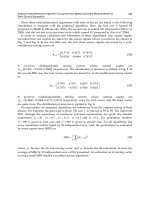
presented in a common foundation. Figure 1 shows an example of the most general MIMO
acoustical scenario.


Fig. 1. Audio application scenario.
(
)
ns
2
(
)
ns
I
(
)
nx
1
(
)

nx
2
(
)
nx
P
()
ns
1
(
)
nr
()
ny
1
()
ny
2
()
ny
O
W
V
New Developments in Robotics, Automation and Control

28
The box, on the left, represents a reverberant room.
V is a L
I
P

×
matrix that contains the
acoustic impulse responses (AIR) between the
I
sources and
P
microphones (channels);
L

is a filters length. Sources can be interesting or desired signals (to enhance) or noise and
interference (to attenuate). The discontinuous lines represent only the direct path and some
first reflections between the
(
)
ns
1
source and the microphone with output signal
()
nx
1
. Each
()
n
pi
v vector represents the AIR between Ii K1
=
and Pp K1
=
positions and is constantly
changing depending on the position of both: source or microphone, angle between them,

radiation pattern, etc.

⎥
⎥
⎥
⎥
⎥
⎦
⎤
⎢
⎢
⎢
⎢
⎢
⎣
⎡
=
PIPP
I
I
vvv
vvv
vvv
V
L
MOMM
L
L
21
22221

11211
,

v
pi
=[ v
pi1
v
pi2 ···
v
piL
].

(1)

()
nr is an additive noise or interference signal.
(
)
nx
p
,
Pp K1=
is a corrupted or poor quality
signal that wants to be improved. The filtering goal is to obtain a
W
matrix so that
() ()
nsny
io

ˆ
≈ corresponds to the identified signal. The signals in the Fig. 1 are related by

(
)
(
)
(
)
nrnn += Vsx
,
(2)
y(n) = Wx(n).

(3)

()
ns is a
1×LI
vector that collects the source signals,

() () () ()
[
]
T
T
I
TT
nnnn ssss L
21

=
,
(4)
()
(
)
(
)
(
)
[
]
T
iiii
Lnsnsnsn 11 +−−= Ls
.


()
nx is a 1×P vector that corresponds to the convolutive system output excited by
()
ns
and the adaptive filter input of order
LPO
×
.
(
)
nx
p

is an input corresponding to the channel
p
containing the last L samples of the input signal x ,

() () () ()
[
]
T
T
P
TT
nnnn xxxx L
21
=
,
(5)
x
p
(n)=[ x
p
(n) x
p
(n-1)
···
x
p
(n-L+1)]
T
.

Multichannel Speech Enhancement

29
W
is an LPO× adaptive matrix that contains an AIRs between the P inputs andO outputs
⎥
⎥
⎥
⎥
⎥
⎦
⎤
⎢
⎢
⎢
⎢
⎢
⎣
⎡
=
OPOO
P
P
www
www
www
W
L
MOMM

L
L
21
22221
11211
,

w
op
= [w
op1
w
op2 ···
w
opL
].

(6)

For a particular output Oo K1
=
, normally matrix
W
is rearranged as column vector

[
]
T
P
wwww L

21
= .
(7)

Finally,
()
ny is an 1
×
O target vector,
(
)()
(
)
(
)
[
]
T
O
nynynyn L
21
=y .
The used notation is the following:
a or
α
is a scalar, a is a vector and
A
is a matrix in
time-domain
a is a vector and

A
is a matrix in frequency-domain. Equations (2) and (3) are
in matricial form and correspond to convolutions in a time-domain. The index
n
is the
discrete time instant linked to the time (in seconds) by means of a sample frequency
s
F
according to
s
nTt = ,
ss
FT 1
=
.
s
T is the sample period. Superscript
T
denotes the transpose
of a vector or a matrix,
∗
denotes the conjugate of a vector or a matrix and superscript
H

denotes Hermitian (the conjugated transpose) of a vector or a matrix. Note that, if adaptive
filters are
1×L vectors, L samples have to be accumulated per channel (i.e. delay line) to
make the convolutions (2) and (3).
The major assumption in developing linear time-invariant (LTI) systems is that the
unwanted noise can be modeled by an additive Gaussian process. However, in some

physical and natural systems, noise can not be modelled simply as an additive Gaussian
process, and the signal processing solution may also not be readily expressed in terms of
mean squared errors (MSE)
1
.
From a signal processing point of view, the particular problem of noise reduction generally
involves two major steps:
modeling and filtering. The modelling step generally involves
determining some approximations of either the noise spectrum or the input signal spectrum.
Then, some filtering is applied to emphasize the signal spectrum or attenuate/reject the
noise spectrum (Chau, 2001). Adaptive filtering techniques are used largely in audio
applications where the ambient noise environment has a complicated spectrum, the statistics
are rapidly varying and the filter coefficients must automatically change in order to
maintain a good intelligibility of the speech signal. Thus, filtering techniques must be

1
MSE is the best estimator for random (or stochastic) signals with Gaussian distribution (normal
process). The Gaussian process is perhaps the most widely applied of all stochastic models: most error
processes, in an estimation situation, can be approximated by a Gaussian process; many non-Gaussian
random processes can be approximated with a weighted combination of a number of Gaussian densities
of appropriated means and variances; optimal estimation methods based on Gaussian models often
result in linear and mathematically tractable solutions and the sum of many independent random
process has a Gaussian distribution (central limit theorem) (Vaseghi, 1996).
New Developments in Robotics, Automation and Control

30
powerful, precise and adaptive. Most non-referenced noise reduction systems have only one
single input signal. The task of estimating the noise and/or signal spectra must then make
use of the information available only from the single input signal and the noise reduction
filter will also have only the input signal for filtering.

Referenced adaptive noise
reduction/cancellation systems work well only in constrained environments where a good
reference input is available, and the crosstalk problem is negligible or properly addressed.

2. Multichannel Adaptive Filters

In a multichannel system ( 1>P ) it is possible to remove noise and interference signals by
applying sophisticated adaptive filtering techniques that use spatial or redundant
information. However there are a number of noise and distortion sources that can not be
minimized by increasing the number of microphones. Examples of this are the surveillance,
recording, and playback equipment. There are several classes of adaptive filtering (Honig &
Messerschmitt, 1984) that can be useful for speech enhancement, as will be shown in Sect. 4.
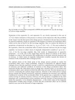
The differences among them are based on the external connections to the filter. In the
estimator application [see Fig. 2(a)], the internal parameters of the adaptive filter are used as
estimate. In the predictor application [see Fig. 2(b)], the filter is used to filter an input signal,
()
nx , in order to minimize the output signal,
(
)
(
)
(
)
nynxne
−
=
, within the constrains of the
filter structure. A
predictor structure is a linear weighting of some finite number of past input
samples used to estimate or predict the current input sample. In the joint-process estimator

application [see Fig. 2(c)] there are two inputs,
(
)
nx and
(
)
nd . The objective is usually to
minimize the size of the output signal,
(
)
(
)
(
)
nyndne
−
=
, in which case the objective of the
adaptive filter itself is to generate an estimate of
(
)
nd , based on a filtered version of
()
nx ,
()
ny (Honig & Messerschmitt, 1984).


Fig. 2. Classes of adaptive filtering.
(a)

(b)
(c)
Adaptive

filter
Adaptive

filter
Adaptive

filter
Parameters

(
)
nx
(
)
nx
(
)
nx
(
)
ny
(
)
ne
(
)

ne
(
)
ny
(
)
nd
Multichannel Speech Enhancement

31
2.1 Filter Structures
Adaptive filters, as any type of filter, can be implemented using different structures. There
are three types of
linear filters with finite memory: the transversal filter, lattice predictor and
systolic array (Haykin, 2002).

2.1.1 Transversal
The
transversal filter, tapped-delay line filter or finite-duration impulse response filter (FIR) is the
most suitable and the most commonly employed structure for an adaptive filter. The utility
of this structure derives from its simplicity and generality.
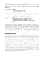
The multichannel transversal filter output used to build a joint-process estimator as
illustrated in Fig. 2(c) is given by

() ( ) () ()
11 1
1, ,
PL P
pl p p p
pl p

yn wx n l n n
== =
=−+= =
∑∑ ∑
wx wx .
(8)

Where
(
)
nx
is defined in (5) and
w
in (7). Equation (8) is called finite convolution sum.


Fig. 3. Multichannel transversal adaptive filtering.

2.1.2 Lattice
The
lattice filter is an alternative to the transversal filter structure for the realization of a
predictor (Friedlander, 1982).
(
)
nd
(
)
ne
(
)

ny
(
)
ny
1
(
)
ny
P
(
)
nx
1
(
)
nx
P
1−
z
1−
z
1−
z
1−
z
1−
z
1−
z
11

w
12
w
L
w
1
1
P
w
2P
w
PL
w
P
w
1
w
New Developments in Robotics, Automation and Control

32

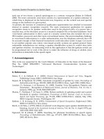
Fig. 4. Multichannel adaptive filtering with lattice-ladder joint-process estimator.

The multichannel version of lattice-ladder structure (Glentis et al., 1999) must consider
the interchannel relationship of the reflection coefficients in each stage
l .

(
)
(

)
(
)()
(
)
111
1,
∗
−−
=+ − =
ll ll
nn nnnff Kb fx
,
(9)
(
)
(
)
(
)
(
)
(
)
111
1,
ll ll
nn nnn
−−
=−+ =bb Kfbx.

(10)

Where
() ()
(
)
(
)
[]
T
Pllll
nfnfnfn L
21
=f ,
(
)
(
)
(
)
(
)
[]
T
Pllll
nbnbnbn L
21
=b ,

() () ()
(
)
[]
T
P
nxnxnxn L
21
=x , and

T
PPllPlP
Plll
Plll
l
kkk
kkk
kkk
⎥
⎥
⎥
⎥
⎥
⎦
⎤
⎢
⎢
⎢
⎢
⎢

⎣
⎡
=
L
MOMM
L
L
21
22221
11211
K .

The joint-process estimation of the lattice-ladder structure is especially useful for the adaptive
filtering because its predictor
diagonalizes completely the autocorrelation matrix. The transfer
function of a lattice filter structure is more complex than a transversal filter because the
reflexion coefficients are involved,

()
nx
1
()
nx
P
(
)
ne
(
)
nd

(
)
ny
(
)
ny
1
(
)
ny
P
()
nf
11
()
nb
11
1−
z
11
w
(
)
nf
12
(
)
nb
12
1−

z
12
w
()
(
)
nf
L 11 −
()
(
)
nb
L 11 −
(
)
nf
L1
(
)
nb
L1
1−
z
()
11 −L
w
L
w
1
()

nf
P1
()
nb
P1
1−
z
1P
w
(
)
nf
P2
(
)
nb
P2
1−
z
2P
w
()
(
)
nf
LP 1−
()
(
)
nb

LP 1−
(
)
nf
PL
(
)
nb
PL
1−
z
()
1−LP
w
PL
w
Multichannel Speech Enhancement

33
(
)
(
)
(
)
1
1nn n=−+bAb Kf
, (11)
(
)

(
)
(
)
1
1yn n n=−+wAb wKf
.

(12)

Where
[]
T
T
L
TT
wwww L
21
= is a 1
×
LP vector of the joint-process estimator coefficients,
[]
T
Pllll
www L
21
=w .
() () () ()
[
]

T
T
L
TT
nnnn bbbb L
21
=
is a
1×LP
backward predictor
coefficients vector. A is a LPLP× matrix obtained with a recursive development of (9) and
(10),


P
P×
I
is a matrix with only ones in the main diagonal and
P
P
×
0
is a
PP ×
zero matrix.
[]
12 1
T
PP L×−
=KI KK KL is a PLP

×
reflection coefficients matrix.

2.2 Adaptation Algorithms
Once a filter structure has been selected, an
adaptation algorithm must also be chosen. From
control engineering point of view, the speech enhancement is a system identification
problem that can be solved by choosing an optimum criteria or cost function
()
wJ in a block
or
recursive approach. Several alternatives are available, and they generally exchange
increased complexity for improved performance (speed of adaptation and accuracy of the
transfer function after adaption or misalignment defined by
22
vwv −=
ε
).

2.2.1 Cost Functions
Cost functions are related to the statistics of the involved signals and depend on some error
signal

(
)
(
)
{
}
nefJ

=
w
.
(14)
The error signal
(
)
ne depends on the specific structure and the adaptive filtering strategy
but it is usually some kind of similarity measure between the target signal
()
ns
i
and the
12
13 23
13 23
12 22
11 21 21
×× × ××
×× × ××
∗
××××
∗∗
×××
∗∗
−− × ××
∗∗
−− × ××
∗∗ ∗
−− −−××

⎡⎤
⎢⎥
⎢⎥
⎢⎥
⎢⎥
⎢
=
⎢
⎢
⎢
⎢
⎢
⎢
⎣⎦
L
L
L
L
MMOM MM
L
L
L
P
PPP PP PPPP
P
PPP PP PPPP
P
PPPPPPP
P
PPPPP

L
LPPPPPP
L
LPPPPPP
L
LLLPPPP
00 0 00
I0 0 00
KK I 0 0 0
KK KK 0 0 0
A
KK KK 0 0 0
KK KK I 0 0
KK KK K K I 0
⎥
⎥
⎥
⎥
⎥
⎥
⎥
.
(13)
New Developments in Robotics, Automation and Control

34
estimated signal
(
)
(

)
nsny
io
ˆ
≈ , for OI
=
. The most habitual cost functions are listed in
Table1.

()
wJ
Comments
()
2
ne
Mean squared error (MSE). Statistic mean operator
(
)
∑
−1
2
1
N
ne
N

MSE estimator. MSE is normally unknown
()
ne
2

Instantaneous squared error
()
ne
Absolute error. Instantaneous module error
(
)
∑
−
n
mn
me
2
λ

Least squares (Weighted sum of the squared error)
() ()
{
}
22
nnE
ll
bf +
Mean squared predictor errors (for a lattice structure)
Table 1. Cost functions for adaptive filtering.

2.2.2 Stochastic Estimation
Non-recursive or block methods apply batch processing to a transversal filter structure. The
input signal is divided into time blocks, and each block is processed independently or with
some overlap. This algorithms have

finite memory.
The use of memory (vectors or matrice blocks) improves the benefits of the adaptive
algorithm because they emphasize the variations in the crosscorrelation between the
channels. However, this requires a careful structuring of the data, and they also increase the
computational exigencies: memory and processing. For channel
p
, the input signal vector
defined in (5) happens to be a matrix of the form

() ( ) ( )
()
()
111
T
TT T
pp p p
nnN nN n
⎡
⎤
=−+ −−+
⎣
⎦
Xx x xL
,
(15)
()
() ()
(
)
()

() ()
()
()
()()
()
()
111
11
212 1
pp p
pp p
p
pp p
xnN xn N xn
xnN xn N xn
n
xnNL xn N L xnL
⎡⎤
−+ − −+
⎢⎥
−−− −
⎢⎥
=
⎢⎥
⎢⎥
⎢⎥
−−+ − −−+ −+
⎣⎦
X
L

L
MMOM
L
,

() ( ) ( )
()
()
111
T
ndnN dnN dn
⎡
⎤
=−+ −−+
⎣
⎦
d L
,
(16)

where N represents the memory size. The input signal matrix to the multichannel adaptive
filtering has the form

() () () ()
12
T
TT T
P
nnn n
⎡

⎤
=
⎣
⎦
XXX XL
.
(17)

Multichannel Speech Enhancement

35
In the most general case (with order memory
N ), the input signal
(
)
nX
is a matrix of size
NLP× . For 1=N (memoryless) and 1=P (single channel) (17) is reduced to (5).
There are adaptive algorithms that use memory 1
>N to modify the coefficients of the filter,
not only in the direction of the input signal
(
)
nx , but within the hyperplane spanned by the
()
nx and its 1−N immediate predecessors
(
)
(
)

(
)
[
]
11
+
−
−
Nnxnxnx L per channel.
The block adaptation algorithm updates its coefficients once every
N samples as

(
)
(
)
(
)
1mmm+= +Δwww,
(18)

(
)
(
)
arg minmJΔ=ww.


The matrix defined by (15) stores 1
−

+
=
NLK samples per channel. The time index m
makes reference to a single update of the weights from time
n to Nn
+
, based on the
K

accumulated samples.
The stochastic recursive methods, unlike the different optimization deterministic iterative
algorithms, allow the system to approach the solution with the partial information of the
signals using the general rule

(
)
(
)
(
)
1nnn+= +Δwww
,
(19)

(
)
(
)
arg minnJΔ=ww.

The new estimator
(
)
1n
+
w
is updated from the previous estimation
()
nw
plus the
adapting-step or gradient obtained from the cost function minimization
()
J w . These
algorithms have an
infinite memory. The trade-off between convergence speed and the
accuracy is intimately tied to the length of memory of the algorithm. The error of the joint-
process estimator using a transversal filter with memory can be rewritten like a vector as

(
)
(
)
(
)
(
)
(
)
(

)
T
nnnn nn=−=−edydXw.
(20)

The unknown system solution, applying the MSE as the cost function, leads to the normal or
Wiener-Hopf equation. The Wiener filter coefficients are obtained by setting the gradient of
the square error function to zero, this yields

1
1
−
∗−
⎡⎤
==
⎣⎦
H
wXX XdRr.
(21)

R
is a correlation matrix and r is a cross-correlation vector defined by

New Developments in Robotics, Automation and Control

36
11 12 1
21 22 2
12
P

P
H
PP PP
⎡
⎤
⎢
⎥
⎢
⎥
==
⎢
⎥
⎢
⎥
⎣
⎦
XX XX XX
XX XX XX
RXX
XX XX XX
L
L
MMOM
L
,
(22)
12
∗
∗∗∗
⎡

⎤
==
⎣
⎦
L
T
P
rXd Xd Xd Xd .
(23)

For each Ii K1= input source,
(
)
21
−
PP relations are obtained:
p
H
qq
H
p
wxwx = for
Pqp K1, = , with
q
p
≠
. Given vector
[
]
T

TT
P
p
T
p 11
2
wwwu −−=
∑
=
L , due to the nearness
with which microphones are placed in scenario of Fig. 1, it is possible to verify that
1×
=
PL
0Ru , thus R is not invertible and no unique problem solution exists. The adaptive
algorithm leads to one of many possible solutions which can be very different from the
target
v . This is known as a non-unicity problem.
For a prediction application, the cross-correlation vector
r must be slightly modified as
()
1−= nXxr ,
()
(
)
(
)
(
)
[

]
T
Nnxnxnxn −−−=− L211x and
1=P
.
The optimal Wiener-Hopf solution
rRw
1
opt
−
= requires the knowledge of both magnitudes:
the correlation matrix
R
of the input matrix
X
and the cross-correlation vector r between
the input vector and desired answer
d . That is the reason why it has little practical value. So
that the linear system given by (21) has solution, the correlation matrix
R must be
nonsingular. It is possible to estimate both magnitudes according to the windowing method
of the input vector.
The sliding window method uses the sample data within a window of finite length N .
Correlation matrix and cross-correlation vector are estimated averaging in time,

(
)
(
)
(

)
Nnnn
H
XXR = ,
(24)

(
)
(
)
(
)
Nnnn
∗
= dXr .


The method that estimates the autocorrelation matrix like in (24) with samples organized as
in (15) is known as the
covariance method. The matrix that results is positive semidefinite but
it is not Toeplitz.
The
exponential window method uses a recursive estimation according to certain forgetfulness
factor
λ
in the rank 10
<
<
λ
,

(
)
(
)
(
)
(
)
nnnn
H
XXRR +−= 1
λ
,
(25)

(
)
(
)
(
)
(
)
nnnn
∗
+−= dXrr 1
λ
.

Multichannel Speech Enhancement

37
When the excitation signal to the adaptive system is not stationary and the unknown system
is time-varying, the exponential and sliding window methods allow the filter to forget or to
eliminate errors happened farther in time. The price of this forgetfulness is deterioration in
the fidelity of the filter estimation (Gay & Benesty, 2000).
A recursive estimator has the form defined in (19). In each iteration, the update of the
estimator is made in the
(
)
nΔw direction. For all the optimization deterministic iterative
schemes, a stochastic algorithm approach exists. All it takes is to replace the terms related to
the cost function and calculate the approximate values by each new set of input/output
samples. In general, most of the adaptive algorithms turn a stochastic optimization problem
into a deterministic one and the obtained solution is an approximation to the one of the
original problem.

The gradient
()
(
)
22
∗
∂
=∇ = =− +
∂
H
J

J
w
g w Xd XX w
w
, can be estimated by means of
()
2=− +grRw, or by the equivalent one
∗
=−
g
Xe
, considering
R
and r according to (24)
or (25). It is possible to define recursive updating strategies, per each
l stage, for lattice
structures as

(
)
(
)
(
)
1
lll
nnn+= +ΔKKK
,
(26)

(
)
(
)
arg min
ll
nJΔ=KK.


2.2.3 Optimization strategies
Several strategies to solve
(
)
arg min JΔ=ww are proposed (Glentis et al., 1999) (usually of
the least square type). It is possible to use a quadratic (second order) approximation of the
error-performance surface around the current point denoted
(
)
nw
. Recalling the second-
order
Taylor series expansion of the cost function
(
)
J w around
(
)
nw , with
()
nΔ= −www ,

you have

( ) () () ()
+Δ ≅ +Δ ∇ + Δ ∇ Δ
2
1
2
HH
JJ J Jww w w w w ww


(27)

Deterministic iterative optimization schemes require the knowledge of the cost function, the
gradient (first derivatives) defined in (29) or the Hessian matrix (second order partial
derivatives) defined in (45,52) while
stochastic recursive methods replace these functions by
impartial estimations.

()
()
() ()
⎡
⎤
∂∂ ∂
∇=
⎢
⎥
∂∂ ∂
⎣

⎦
L
12
T
L
JJ J
J
ww w
w
ww w
,
(28)
New Developments in Robotics, Automation and Control

38
()
()
() ()
() () ()
() () ()
⎡
⎤
∂∂ ∂
⎢
⎥
∂∂ ∂∂ ∂∂
⎢
⎥
⎢
⎥

∂∂ ∂
⎢
⎥
∇=
∂∂ ∂∂ ∂∂
⎢
⎥
⎢
⎥
⎢
⎥
⎢
⎥
∂∂ ∂
⎢
⎥
∂∂ ∂∂ ∂∂
⎣
⎦
L
L
MMOM
L
22 2
11 12 1
22 2
2
21 22 2
22 2
12

T
L
L
LL LL
JJ J
JJ J
J
JJ J
ww w
ww ww ww
ww w
w
ww ww ww
ww w
ww ww ww
.
(29)

The vector
(
)
(
)
=∇nJgw is the gradient evaluated at
(
)
nw , and the matrix
(
)
(

)
=∇
2
nJHw
is the
Hessian of the cost function evaluated at
(
)
nw .
Several first order adaptation strategies are: to choose a starting initial point
(
)
0w , to
increment election
(
)
(
)
(
)
μ
Δ=nnnwg; two decisions are due to take: movement direction
(
)
ng in which the cost function decreases fastest and the step-size in that direction
()
μ
n .
The iteration stops when a certain level of error is reached
(

)
ξ
Δ
<nw ,

(
)
(
)
(
)
(
)
1nnnn
μ
+= +ww g
.
(30)

Both parameters
(
)
n
μ
,
(
)
ng
are determined by a cost function. The second order methods
generate values close to the solution in a minimum number of steps but, unlike the first

order methods, the second order derivatives are very expensive computationally. The
adaptive filters and its performance are characterized by a selection criteria of
(
)
n
μ
and
(
)
ng parameters.

Method Definition Comments
SD
()
2
H
n
μ
=−
g
gRg

Steepest-Descent
CG (See below) Conjugate Gradient
NR
(
)
n
μ
α

= Q

Newton-Raphson
Table 2. Optimization methods.

The optimization methods are useful to find the minimum or maximum of a quadratic
function. Table 2 summarizes the optimization methods. SD is an iterative optimization
procedure of easy implementation and computationaly very cheap. It is recommended with
cost functions that have only one minimum and whose gradients are isotropic in magnitude
respect to any direction far from this minimum. NR method increases SD performance using
a carefully selected weighting matrix. The simplest form of NR uses
1
−
=QR. Quasy-Newton
Multichannel Speech Enhancement

39
methods (QN) are a special case of NR with
Q
simplified to a constant matrix. The solution
to
()
J w is also the solution to the normal equation (21). The conjugate gradient (CG) (Boray &
Srinath, 1992) was designed originally for the minimization of convex quadratic functions
but, with some variations, it has been extended to the general case. The first CG iteration is
the same that the SD algorithm and the new successive directions are selected in such a way
that they form a set of vectors mutually conjugated to the Hessian matrix (corresponding to
the autocorrelation matrix,
R ), 0,
H

ij
ij
=
∀≠qRq . In general, CG methods have the form

1
,1
,1
l
l
lll
l
l
β
−
−
=
⎧
=
⎨
−
+>
⎩
g
q
gq

(31)
,
,

ll
l
ll l
μ
=
−
gq
qg p
,
(32)
2
2
1
l
l
l
β
−
=
g
g
,
(33)
(
)
(
)
(
)
1llll

nnn
μ
+
=+ww q.
(34)
CG spans the search directions from the gradient in course,
g , and a combination of
previous
R -conjugated search directions.
β
guarantees the R -conjugation. Several
methods can be used to obtain
β
. This method (33) is known as Fleetcher-Reeves. The
gradients can be obtained as
(
)
=∇Jgw and
(
)
=∇ −Jpwg.
The
memoryless LS methods in Table 3 use the instantaneous squared error cost function
() ()
=
2
Jenw . The descent direction for all is a gradient
(
)
(

)
(
)
nnen
∗
=gx . The LMS
algorithm is a stochastic version of the SD optimization method. NLMS frees the
convergence speed of the algorithm with the power signal. FNLMS filters the signal power
estimation; 01
β
<< is a weighting factor. PNLMS adaptively controls the size of each
weight.

Method Definition Comments
LMS
(
)
n
μ
α
=

Least Means Squares
NLMS
()
()
2
n
n
α

μ
δ
=
+
x

Normalized LMS
FNLMS
()
()
n
n
α
μ
=
p

Filtered NLMS
PNLMS
()
() ()
H
n
nn
α
μ
δ
=
+
Q

xQx

Proportionate NLMS
Table 3. Memoryless Least-Squares (LS) methods.
New Developments in Robotics, Automation and Control

40
Method Definition Comments
RLS
(
)
(
)
1
nn
μ
−
=R

(
)
(
)
(
)
nnen
∗
=gx

Recursive Least-Squares
LMS-SW
()
()
() () ()()
2
HH
n
n
nn nn
μ
δ
=
+
g
gXXg

(
)
(
)
(
)
=
*
nnengX


Sliding-Window LMS
APA

()
() ()
H
n
nn
α
μ
δ
=
+XX I

(
)
(
)
(
)
nnen
∗
=gX


Affine Projection Algorithm
PRA
(
)
(
)
(
)

(
)
11nnNnn
μ
+= −++ww g

()
() ()
H
n
nn
α
μ
δ
=
+XX I

(
)
(
)
(
)
nnen
∗
=gX


Partial Rank Algorithm
DLMS

()
() ()
1
,
n
nn
μ
=
xz

(
)
(
)
(
)
=
*
nnengz

() ()
(
)
(
)
()
()
−
=
+−

−
2
,1
1
1
nn
nn n
n
xx
zx x
x



Decorrelated LMS
TDLMS
()
()
α
μ
=
2
n
n
Q
x
,
=
1
H

QQ

(
)
(
)
(
)
nnen
∗
=gx



Transform-Domain DLMS
Table 4. Least-Squares with memory methods.

Q is a diagonal matrix that weights the individual coefficients of the filters,
α
is a relaxation
constant
and
δ
guarantees that the denominator never becomes zero. These algorithms are
very cheap computationally but their convergence speed depends strongly on the
spectral
condition number
of the autocorrelation matrix
R
(that relate the extreme eigenvalues) and

can get to be unacceptable as the correlation between the
P channels increases.
Multichannel Speech Enhancement

41
The projection algorithms in Table 4 modify the filters coefficients in the input vector direction
and on the subspace spanned by the 1
−
N redecessors. RLS is a recursive solution to the
normal equation that uses MSE as cost function. There is an alternative fast version FRLS.
LMS-SW is a variant of SD that considers a data window. The step can be obtained by a
linear search. APA is a generalization of RLS and NLMS. APA is obtained by projecting the
adaptive coefficients vector
w in the affine subspace. The affine subspace is obtained by
means of a translation from the orthogonal origin to the subspace where the vector
w is
projected. PRA is a strategy to reduce the computational complexity of APA by updating the
coefficients every
N samples. DLMS replaces the system input by an orthogonal component
to the last input (order 2). These changes the updating vector direction of the correlated
input signals so that these ones correspond to uncorrelated input signals. TDLMS
decorrelates into transform domain by means of a
Q matrix.
The adaptation of the transversal section of the joint-process estimator in the lattice-ladder
structure depends on the gradient
(
)
ng and, indirectly, on the reflection coefficients,
through the backward predictor,
(

)
(
)
=nngb. However, the reflection coefficient adaptation
depends on the gradient of
(
)
y
n with respect to them

()
()
() ()
⎡
⎤
∂∂ ∂
∇=
⎢
⎥
∂∂ ∂
⎣
⎦
L
12
T
L
JJ J
J
KK K
K

KK K
,
(35)
()
()
() ()
() () ()
() () ()
⎡
⎤
∂∂ ∂
⎢
⎥
∂∂ ∂∂ ∂∂
⎢
⎥
⎢
⎥
∂∂ ∂
⎢
⎥
∇=
∂∂ ∂∂ ∂∂
⎢
⎥
⎢
⎥
⎢
⎥
⎢

⎥
∂∂ ∂
⎢
⎥
∂∂ ∂∂ ∂∂
⎣
⎦
L
L
MMOM
L
22 2
11 12 1
22 2
2
21 22 2
22 2
12
L
L
LL LL
JJ J
JJ J
J
JJ J
KK K
KK KK KK
KK K
K
KK KK KK

KK K
KK KK KK
.
(36)

In a more general case, concerning to a multichannel case, the gradient matrix can be
obtained as
(
)
=∇JGK. Two recursive updatings are necessary

(
)
(
)
(
)
(
)
1
llll
nnnn
μ
+= +ww g
,
(37)
(
)
(
)

(
)
(
)
1
llll
nnnn
λ
+= +KK G

(38)

Table 5 resumes the least-squares for lattice.
GAL is a NLMS extension for a lattice structure that uses two cost functions: instantaneous
squared error for the tranversal part and prediction MSE for the lattice-ladder part,
() ( ) ( ) () ()
(
)
22
11 1
ll ll
nn nn
ββ
=−+− +−BB fb , where
α
and
σ
are relaxation factors.
New Developments in Robotics, Automation and Control

42
Method Definition Comments
GAL
()
()
2
α
μ
=
l
l
n
nb

(
)
(
)
(
)
ll
nnen
∗
=gb

()
()
1
l
l

n
n
σ
λ
−
=
B

(
)
(
)
(
)
(
)
(
)
11
11
HH
ll l ll
nnnnn
−−
=
−+ −Gb f bf

Gradient Adaptive Lattice
CGAL
(See below)

CG Adaptive Lattice
Table 5. Least-Squares for lattice.

For CGAL, the same algorithm described in (31-34) is used but it is necessary to rearrange
the gradient matrices of the lattice system in a column vector. It is possible to arrange the
gradients of all lattice structures in matrices.
() () () ()
12
T
TT T
P
nnn n
⎡
⎤
=
⎣
⎦
Ugg gL
is the
LP× gradient matrix with respect to the transversal coefficients,
()
12
T
ppp pL
ngg g
⎡⎤
=
⎣⎦
g L , Pp K1
=

.
() () () ()
12
T
P
nnn n=
⎡
⎤
⎣
⎦
VGG GL
is a
()
PLP 1−× gradient matrix with respect to the reflection coefficients; and rearranging these
matrices in one single column vector,
T
TT
⎡
⎤
⎣
⎦
uv is obtained with
[]
11 1 21 2 1
T
LLPPL
gggggg=u LLLL,
()
111 1 1 11 1 112
1

T
PP PP
PP L
GG G GGG
−
⎡
⎤
=
⎣
⎦
v LLL L
.

1
,1
,1
l
l
lll
l
l
β
−
−
=
⎧
=
⎨
−
+>

⎩
g
q
gq

(39)
()
T
T
T
T
1
,1
1,1
αα
−
⎧
⎡⎤
=
⎪⎣ ⎦
=
⎨
⎪
⎡⎤
+
−>
⎣⎦
⎩
T
l

T
l
l
l
uv
g
guv

(40)
2
2
1
l
l
l
β
−
=
g
g
,
(41)
w
l+1
= w
l
+ μ u
l
,

(42)
1
λ
+
=
+
llll
KKV
.
(43)
Multichannel Speech Enhancement

43
The time index n has been removed by simplicity. 10
<
<
α
is a forgetfulness factor which
weights the innovation importance specified in a low-pass filtering in (40). The gradient
selection is very important. A mean value that uses more recent coefficients is needed for
gradient estimation and to generate a vector with more than one conjugate direction (40).

3. Multirate Adaptive Filtering

The adaptive filters used for speech enhancement are probably very large (due to the AIRs).
Multirate adaptive filtering works at a lower sampling rate that allows reducing the
complexity (Shynk, 1992). Depending on how the data and filters are organized, these
approaches may upgrade in performance and avoid end-to-end delay. Multirate schemes
adapt the filters in smaller sections at lower computational cost. This is only necessary for
real-time implementations. Two approaches are considered. The

subband adaptive filtering
approach splits the spectra of the signal in a number of subbands that can be adapted
independently and afterwards the filtering can be carried out in a fullband. The
frequency-
domain adaptive filtering
partitions the signal in time-domain and projects it into a
transformed domain (i.e. frequency) using better properties for adaptive processing. In both
cases the input signals are transformed into a more desirable form before adaptive
processing and the adaptive algorithms operate in transformed domains, whose basis
functions orthogonalize the input signal, speeding up the convergence. The
partitioned
convolution
is necessary for fullband delayless convolution and can be seen as an efficient
frequency-domain convolution.

3.1 Subband Adaptive Filtering
The fundamental structure for subband adaptive filtering is obtained using band-pass filters
as basis functions and replacing the fixed gains for adaptive filters. Several implementations
are possible. A typical configuration uses an
analysis filter bank, a processing stage and a
synthesis filter bank. Unfortunately, this approach introduces an end-to-end delay due to the
synthesis filter bank. Figure 5 shows an alternative structure which adapts in subbands and
filters in full-band to remove this delay (Reilly et al., 2002).
K
is the decimation ratio, M is the number of bands and N is the prototype filter length. k
is the low rate time index. The sample rate in subbands is reduced to
KF
s
. The input signal
per channel is represented by a vector

() () ( ) ( )
11
T
p
nxnxn xnL=− −+
⎡
⎤
⎣
⎦
x
L
,
Pp K1=
. The adaptive filter in full-band per channel
12
T
ppp PL
ww w
⎡
⎤
=
⎣
⎦
w L
is
obtained by means of the
T operator as

()
2

1
K
M
pmpmm
K
m
↓
↑
=
⎧
⎫
=ℜ ∗ ∗
⎨
⎬
⎩⎭
∑
whw
g
,
(44)

from the subband adaptive filters per each channel
p
m
w , Pp K1
=
, 21 Mm K
=
(Reilly et
al., 2002). The subband filters are very short, of length

1
1
LN N
C
KK
+−
⎡⎤⎡⎤
=
−+
⎢⎥⎢⎥
⎢⎥⎢⎥
, which
New Developments in Robotics, Automation and Control

44
allows to use much more complex algorithms. Although the input signal vector per channel
()
p
nx has size 1
×
L , it acts as a delay line which, for each iteration k , updates K samples.
K↓ is an operator that means downsampling for a K factor and K
↑
upsampling for a K
factor.
m
g is a synthesis filter in subband m obtained by modulating a prototype filter. H
is a
polyphase matrix of a generalized discrete Fourier transform (GDFT) of an oversampled
(

MK < ) analysis filter bank (Crochiere & Rabiner, 1983). This is an efficient implementation
of a uniform complex modulated analysis filter bank. This way, only a
prototype filter p is
necessary; the prototype filter is a low-pass filter.
The band-pass filters are obtained modulating a prototype filter. It is possible to select
different adaptive algorithms or parameter sets for each subband. For delayless
implementation, the full-band convolution may be made by a
partitioned convolution.


Fig. 5. Subband adaptive filtering. This configuration is known as
open-loop because the error
is in the time-domain. An alternative
closed-loop can be used where the error is in the
subband-domain. Gray boxes correspond to efficient polyphase implementations. See
details in (Reilly et al., 2002).
Multichannel Speech Enhancement

45
3.2 Frequency Domain Adaptive Filtering
The basic operation in frequency-domain adaptive filtering (FDAF) is to transform the input
signal in a “more desirable” form before the adaptation process starts (Shynk, 1992) in order
to work with matrix multiplications instead of dealing with slow convolutions.
The frequency-domain transform employs one or more
discrete Fourier transforms (DFT), T
operator in Fig. 6, and can be seen as a pre-processing block that generates decorrelated
output signals. In the more general FDAF case, the output of the filter in the time-domain (3)
can be seen as the direct frequency-domain translation of the block LMS (BLMS) algorithm.
That efficiency is obtained taking advantage of the equivalence between the linear
convolution and the circular convolution (multiplication in the frequency-domain).

Fig. 6. Partitioned block frequency-domain adaptive filtering.

It is possible to obtain the linear convolution between a finite length sequence (filter) and an
infinite length sequence (input signal) with the overlapping of certain elements of the data
sequence and the retention of only a subgroup of the DFT.
The
partitioned block frequency-domain adaptive filtering (PBFDAF) was developed to deal
efficiently with such situations (Paez & Otero, 1992). The PBFDAF is a more efficient
implementation of the LMS algorithm in the frequency-domain. It reduces the
computational burden and bounds the user-delay. In general, the PBFDAF is widely used
due to its good trade-off between speed, computational complexity and overall latency.
New Developments in Robotics, Automation and Control

46
However, when working with long AIRs, the convergence properties provided by the
algorithm may not be enough. This technique makes a sequential partition of the impulse
response in the time-domain prior to a frequency-domain implementation of the filtering
operation.
This time segmentation allows setting up individual coefficient updating strategies
concerning different sections of the adaptive canceller, thus avoiding the need to disable the
adaptation in the complete filter. In the PBFDAF case, the filter is partitioned transversally
in an equivalent structure. Partitioning
p
w in
Q
segments ( K length) we obtain

()

()
()
1
11 0
Q
PK
p
pq
Km
pqm
yn x n qK mw
−
+
== =
=−−
∑∑∑
,
(45)

Where the total filter length L , for each channel, is a multiple of the length of each segment
QKL = , LK ≤ . Thus, using the appropriate data sectioning procedure, the Q linear
convolutions (per channel) of the filter can be independently carried out in the frequency-
domain with a total delay of
K samples instead of the QK samples needed by standard
FDAF implementations. Figure 6 shows the block diagram of the algorithm using the
overlap-save method. In the frequency-domain with matricial notation, (45) can be
expressed as

=
⊗

Y
XW
,
(46)

where
X=FX
represents a matrix of dimensions
PQM
×
×
which contains the Fourier
transform of the
Q partitions and
P
channels of the input signal matrix
X
.
F
represents
the DFT matrix defined as
−
=
mn
M
WF
of size MM × and
1
−
F as its inverse. Of course, in the

final implementation, the DFT matrix should be substituted by much more efficient
fast
Fourier transform
(FFT). Being
X
, PK
×
2 -dimensional (supposing 50% overlapping between
the new block and the previous one). It should be taken into account that the algorithm
adapts every
K samples.
W
represents the filter coefficient matrix adapted in the
frequency-domain (also
PQM
×
×
-dimensional) while the
⊗
operator multiplies each of
the elements one by one; which, in (46), represents a
circular convolution. The output vector
y can be obtained as the double sum (rows) of the
Y
matrix. First we obtain a PM ×
matrix which contains the output of each channel in the frequency-domain
y
P
,
Pp K1=

,
and secondly, adding all the outputs we obtain the whole system output,
y . Finally, the
output in the time-domain is obtained by using
1
last components of
−
= yKyF. Notice that the
sums are performed prior to the time-domain translation. This way we reduce
()()
11 −− QP

FFTs in the complete filtering process. As in any adaptive system the error can be obtained
as

=
−edy

(47)
Multichannel Speech Enhancement

47
with
()( ) ( )
()
111
T
dmK dmK d m K
⎡⎤
=++−

⎣⎦
d
L . The error in the frequency-domain (for
the actualization of the filter coefficients) can be obtained as

1×
⎡
⎤
=
⎢
⎥
⎣
⎦
e
K
0
F
e
.
(48)

As we can see, a block of
K zeros is added to ensure a correct linear convolution
implementation. In the same way, for the block gradient estimation, it is necessary to
employ the same error vector in the frequency-domain for each partition
q
and channel
p
.
This can be achieved by generating an error matrix

E
with dimensions PQM ×× which
contains replicas of the error vector, defined in (48), of dimensions
P and
Q
( ←Ee in the
notation). The actualization of the weights is performed as

(
)
(
)
(
)
(
)
1
μ
+= +WW Gmmmm
.
(49)

The instantaneous gradient is estimated as

∗
=
−⊗GXE
.
(50)

This is the unconstrained version of the algorithm which saves two FFTs from the
computational burden at the cost of decreasing the convergence speed. The constrained
version basically makes a gradient projection. The gradient matrix is transformed into the
time-domain and is transformed back into the frequency-domain using only the first
K

elements of
G as

××
⎡
⎤
=
⎢
⎥
⎣
⎦
G
K
QP
G
F
0
.
(51)

A conjugate gradient version of PBFDAF is possible by transforming the gradient matrix to
vectors and reverse (García, 2006). The vectors
g
and

p
in (31,32) should be changed by
←
ll
gG
,
(
)
=∇
ll
JGW
and
←
ll
p
P
,
(
)
=∇ −
lll
JPWG
, with gradient estimation obtained by
averaging the instantaneous gradient estimates over
N past values
()
1
,,
2
−

−
−
=
=∇ =
∑
llklk
N
ll lk
k
J
N
WX d
GW G
.

3.3 Partitioned Convolution
For each input i , the AIR matrix, V , is reorganized in a column vector
[]
T
P
vvvv L
21
= of size 1
×
=
LPN and initially partitioned in a reasonable number Q
of equally-sized blocks
q
v , Qq K1
=

, of length K . Each of these blocks is treated as a