Pivot Charts
Bạn đang xem bản rút gọn của tài liệu. Xem và tải ngay bản đầy đủ của tài liệu tại đây (234.32 KB, 16 trang )
Pivot Charts
A
fter you create a pivot table, you can create a pivot chart, based on one of the pivot tables in
your workbook. A pivot chart can’t be created on its own; it must be based on a pivot table.
Pivot charts are similar to normal Excel charts, but they have some differences and limitations,
as described in this chapter. Except where noted, the problems in this chapter are based on the
Sales10.xlsx sample file.
10.1. Planning and Creating a Pivot Chart
Problem
The sales manager is preparing for a budget meeting in the East region, and she asked you to
create a pivot chart, to show the sales for each food category at each store.
You created a pivot table on the Region Pivot worksheet, with Store and Category in the
Row Labels area, and Quantity in the Values area. Region is in the Report Filters area, with East
selected from the drop-down list.
You aren’t sure which type of chart will work best, and you’re having trouble arranging the
fields so the chart looks right. The meeting is tomorrow, and you’re running out of time. This
problem is based on the Budget.xlsx sample file.
Solution
When you create a pivot chart, it will use the same layout as the pivot table on which it’s
based.
• Fields in the pivot table’s Row Labels area become the fields on the pivot chart’s
category axis—the horizontal axis across the bottom of a column or line chart.
• Fields in the pivot table’s Column Labels area become legend fields (series) in the pivot
chart—the lines or columns.
• Fields in the pivot table’s Values area become the values in the pivot chart, and they
determine the height of a column, or the position of the point on a line.
• Fields in the pivot table’s Report Filters area continue to act as filters in a pivot chart.
When planning a pivot chart, consider how you want the fields arranged in the chart. If no
fields are in the Column Labels area, the chart will have only one series, representing the fields
in the Row Labels area. In this example, with Store and Category fields in the Row Labels area,
189
CHAPTER 10
a column chart would have one column for each store’s sales in each category. All the columns
would be the same color.
If you move the Store field to the Column Labels area and create a pivot chart, each store
would be a series, with a different colored column for each store. You could compare the sales
of each category, to see which store had the best or worst sales.
If, instead, you move the Category field to the Column Labels area and create a pivot
chart, each category would be a series, with a different colored column for each category. You
could compare the sales at each store, to see which category had the best or worst sales.
In this example, the presentation is to the store managers, who may be interested in how
well their stores are performing, compared to the other stores.
1. In the pivot table, move the Store field to the Column Labels area, and leave the
Category field in the Row Labels area.
2. To create a pivot chart, select a cell in the pivot table, and on the Ribbon, click the
Options tab.
3. In the Tools group, click PivotChart.
4. The Insert Chart dialog box opens, where you can select a chart type and subtype. For
this chart, select a Column chart type, and a Clustered Column subtype, and then click
OK. A column chart is a good choice if you are comparing sets of numbers, as in this
case, where you want to compare the total sales for each category at each store.
This creates a pivot chart on the same worksheet as the pivot table (see Figure 10-1). Each
store is represented by a different color column, with the colors and store numbers shown in
the chart’s legend. The category names appear on the horizontal axis at the bottom of the chart,
and you can see which store had the best or worst sales for each category. The height of each
bar represents the quantity sold in each store, for each category. Because the pivot table is fil-
tered to show the East region’s sales, the pivot chart is also filtered.
Figure 10-1. The pivot chart shows sales per category.
It may take some experimentation, moving the fields to different areas of the pivot chart,
but try to create a chart that presents a limited amount of data, in a clean and simple chart
layout. To see the different layouts available with the Store, Category, and Quantity fields, try
the following:
CHAPTER 10
■
PIVOT CHARTS190
1. With the pivot chart selected, move Store to the Axis Fields (Categories) area, below
Category. This creates one series, with the legend entry of Total. All the columns are
blue, and two sets of labels are on the horizontal axis. The category names are the
outer labels on the axis, and store numbers are the inner labels. This layout lets you
compare the sales for all categories at all stores, but the horizontal axis is crowded,
and the single color makes the chart difficult to read at a glance.
2. Move Store above Category in the Axis Fields (Categories) area. This creates one series,
with blue columns, and the legend entry of Total. The store numbers are the outer
labels on the horizontal axis, and category names are the inner labels. This layout lets
you compare the sales for all stores and all categories, but the horizontal axis is
crowded, and the labels are hard to read.
3. Move Category to the Legend Fields (Series) area. This creates a different colored series
for each category. The store numbers are labels on the horizontal axis, and you can
compare how well the categories sold, within each store.
4. Move Store to the Legend Fields (Series) area, above Category. This creates a different
colored series for each store’s sales of each category. The legend contains a lengthy list
of store and category names, and the chart is crowded and difficult to read.
How It Works
The Insert Chart Type dialog box shows a list of chart types at the left. At the right are the sub-
types available for each chart type. You can point to a subtype and see its name in a tooltip.
Selecting a Chart Type
Unless you changed the setting, the default chart type in Excel is a clustered column chart.
Several chart types are available in Excel:
• Column and bar charts are almost the same, except bars are displayed horizontally
across the chart and columns are vertical. Both of these chart types work well for com-
paring specific values, as you’re doing in your chart.
• Line charts and area charts connect the points that represent values and are good for
illustrating changes over time. The charts are the same, except the area charts are filled
with color.
• Pie charts and doughnut charts show the percentage each value comprises in the overall
total. The pie chart type works well when there is a single series and value, such as total
quantity per region. A doughnut chart can show multiple series.
• Surface charts and radar charts are specialized chart types you can use to show differ-
ences in the data or aggregated data.
■
Note
Although they are available in the list of chart types, you cannot use the X Y (Scatter), Bubble, or
Stock chart types when creating a pivot chart.
CHAPTER 10
■
PIVOT CHARTS 191
Selecting a Chart Subtype
After you select a chart type in the Insert Chart Type dialog box, its default chart subtype is
automatically selected. You can select a different subtype, to meet the requirements of your
current chart. The following are a few of the options:
• Clustered column and bar subtypes are useful if you want to compare the individual
values in a series. In the current example, a clustered column lets you compare the cat-
egory sales at each store, side-by-side.
• Stacked column and bar subtypes combine individual values in a single column or bar,
and they let you compare totals. For example, if you select Stacked Column as the sub-
type for the current chart, with Store in the Axis Fields (Categories) area, and Category
in the Legend Fields (Series) area, the chart will have a single column for each store.
Each category is represented by a different color.
• The 100 percent Stacked column and bar subtypes combine individual values in a
single column or bar that represents 100 percent of each item’s value. This lets you
compare percentages within each item. For example, if you select 100 percent Stacked
Column as the subtype for the current chart, with Store in the Axis Fields (Categories)
area, and Category in the Legend Fields (Series) area, the chart will have a single col-
umn for each store. All the columns are the same height, and within each column, each
category’s color shows its percentage of the store’s sales.
• Line charts and area charts also have stacked and 100 percent stacked subtypes similar
to those for the column and bar charts.
• The remaining chart types have subtypes you can test on your pivot charts. Most of
these, such as Line with Markers or Exploded Pie, are simply a different format, rather
than a different layout of the data.
■
Tip
Avoid using the 3-D chart subtypes, because they distort the representation of the data in your charts.
10.2. Quickly Creating a Pivot Chart
Problem
You frequently create pivot charts using the clustered column chart type, and you would like a
quick way to create one on a chart sheet. You’re tired of navigating through the Ribbon’s tabs,
and performing so many steps, just to create a simple chart. This problem is based on the
Regions.xlsx sample file.
CHAPTER 10
■
PIVOT CHARTS192
Solution
You can press one key on the keyboard, to create a pivot chart on a new chart sheet:
1. Select a cell in the pivot table.
2. On the keyboard, press the F11 key.
A pivot chart is created, on a new chart sheet, in the default chart type and subtype. You
can format the pivot chart, or change its layout, if required.
How It Works
If you have not changed the setting, the default chart type is a clustered column chart. If you
usually select a different chart type, you can set that type as the default. You can also create
your own chart templates, and set one of those as the default.
Setting the Default Chart Type
Follow these steps to change the default chart type:
1. Select an empty cell on any worksheet.
2. On the Ribbon’s Insert tab, click the dialog launcher at the bottom right of the Charts
group.
3. In the Insert Chart dialog box, select the chart type and chart subtype you want to set
as the default type. For example, click Line as the chart type, and then click the Line
subtype (see Figure 10-2).
Figure 10-2. Select a chart type and subtype.
■
Note
The X Y (Scatter), Bubble, and Stock chart types are unavailable when creating a pivot chart. If you
select one of these as the default chart type, you will be unable to create a pivot chart with the F11 shortcut.
4. Click Set as Default Chart, and then click Cancel, to close the dialog box without creat-
ing a chart.
CHAPTER 10
■
PIVOT CHARTS 193
Creating a Chart Template
You can create a chart template that stores all the settings you would like to apply to other
charts. For example, if you frequently create a clustered column chart, change the columns to
green, and then add a title and other formatting, you could save a GreenCluster template. Fol-
low these steps to create a chart template:
1. Create a chart with the chart type, formatting, and layout you want to save as a tem-
plate. The chart can be located on a chart sheet, or on a worksheet.
2. Select the chart, and on the Ribbon’s Design tab, in the Type group, click Save As
Template.
3. In the Save Chart Template dialog box, type a file name for the template, such as
GreenCluster. The file extension, crtx, is automatically added to the file name when it
is saved. Leave the Save In folder unchanged, and your template is saved in the default
folder for chart templates.
4. Click Save, to save the template.
To make the template the default chart type, follow these steps:
1. Select an empty cell in the workbook, and on the Ribbon’s Insert tab, click the dialog
launcher at the bottom right of the Charts group.
2. In the list of chart types, click Templates, and then click your template.
3. Click Set As Default Chart, and then click Cancel, to close the dialog box.
4. If you created a chart as a model for the template, you can delete it—click the chart,
and then press the Delete key.
10.3. Creating a Normal Chart from Pivot Table Data
Problem
The sales manager asked you for a pivot chart that shows the number of days customers wait
for service in the East region. You summarized the data from your company’s service work
orders, with Wait days in the Row Labels area, District in the Report Filters area, and Count of
WO (work orders) in the Values area.
The best chart type for this would be an X Y (Scatter) chart, because the chart will have
numbers on both axes—the number of wait days and the count of work orders. However,
when you try to create the chart, you get an error message that says, “You cannot use an X Y
(Scatter), Bubble, or Stock chart type with a chart that has been created from PivotTable
data. Please select a different chart type.” This problem is based on the WaitDays.xlsx
sample workbook.
Workaround
Although you can’t create some types of charts from pivot table data, you can link the data to
another worksheet, and then use the linked data as the source for a chart.
CHAPTER 10
■
PIVOT CHARTS194