Excel 2010 part 9
Bạn đang xem bản rút gọn của tài liệu. Xem và tải ngay bản đầy đủ của tài liệu tại đây (940.06 KB, 10 trang )
80
22
33
55
66
11
44
4
To format the text as italic,
click the Italic button (
).
5
To format the text as
underline, click the Underline
button (
).
•
Excel applies the effects to the
selected range.
6
Click the Font dialog box
launcher (
).
1
Select the range you want to
format.
2
Click the Home tab.
3
To format the text as bold,
click the Bold button (
).
•
Excel applies the bold effect
to the selected range.
Apply Font Effects
You can improve the look and impact of text in
an Excel worksheet by applying font effects to
a range.
Excel’s font effects include common formatting
such as bold, italic, and underline, which are
available on the Ribbon for easy application.
Excel also offers a dialog box tab that includes
many more font effects, including special
effects such as strikethrough, superscripts,
and subscripts.
In most cases, you should not need to apply
more than one or two font effects at a time. If
you use too many effects, it can make the text
difficult to read.
Apply Font
Effects
07_577639-ch05.indd 8007_577639-ch05.indd 80 3/15/10 2:41 PM3/15/10 2:41 PM
81
Formatting Excel Ranges
CHAPTER
5
77
88
99
Are there any font-related keyboard shortcuts I can use?
Yes. Excel supports the following font shortcuts:
Press To
+
Toggle the selected range as bold
+
Toggle the selected range as italic
+
Toggle the selected range as underline
+
Toggle the selected range as strikethrough
8
To format the text as a
superscript, click Superscript
(
changes to ).
•
To format the text as a
subscript, click Subscript
(
changes to ).
9
Click OK.
Excel applies the font effects.
The Format Cells dialog box
appears with the Font tab
displayed.
7
To format the text as
strikethrough, click
Strikethrough (
changes
to
).
07_577639-ch05.indd 8107_577639-ch05.indd 81 3/15/10 2:41 PM3/15/10 2:41 PM
82
22
33
44
11
4
Click a theme color.
•
Alternatively, click one of
Excel’s standard colors.
•
Excel applies the color to the
range text.
Select a Theme or Standard Color
1
Select the range you want to
format.
2
Click the Home tab.
3
Click in the Font Color
list (
).
Change the Font Color
When you build an Excel worksheet, you can
add visual interest to the sheet text by
changing the font color.
By default, each Excel workbook comes with a
theme applied, and you can change the font
color by applying one of the colors from the
workbook’s theme. You learn more about
workbook themes in Chapter 9.
You can also select a color from Excel’s palette
of standard colors, or from a custom color that
you create yourself.
Change the
Font Color
07_577639-ch05.indd 8207_577639-ch05.indd 82 3/15/10 2:41 PM3/15/10 2:41 PM
83
Formatting Excel Ranges
CHAPTER
5
11
55
66
22
33
44
How can I make the best use of fonts in my documents?
•
Do not use many different typefaces in a single document. Stick to one, or at
most two, typefaces to avoid the ransom note look.
•
Avoid overly decorative typefaces because they are often difficult to read.
•
Use bold only for document titles, subtitles, and headings.
•
Use italics only to emphasize words and phrases, or for the titles of books
and magazines.
•
Use larger type sizes only for document titles, subtitles, and, possibly, the
headings.
•
If you change the text color, be sure to leave enough contrast between the
text and the background. In general, dark text on a light background is the
easiest to read.
The Colors dialog box appears.
5
Click the color you want
to use.
•
You can also click the Custom
tab and then either click the
color you want or enter the
values for the Red, Green, and
Blue components of the color.
6
Click OK.
Excel applies the color to the
selected range.
Select a Custom Color
1
Select the range you want to
format.
2
Click the Home tab.
3
Click in the Font Color
list (
).
4
Click More Colors.
07_577639-ch05.indd 8307_577639-ch05.indd 83 3/15/10 2:42 PM3/15/10 2:42 PM
84
11
22
33
Align Text Horizontally
1
Select the range you want to
format.
2
Click the Home tab.
3
In the Alignment group, click
the horizontal alignment
option you want to use:
Click Align Text Left ( ) to
align data with the left side of
each cell.
Click Center ( ) to align data
with the center of each cell.
Click Align Text Right ( ) to
align data with the right side
of each cell.
Excel aligns the data
horizontally within each
selected cell.
•
In this example, the data in
the cells is centered.
Align Text Within a Cell
You can make your worksheets easier to read
by aligning text and numbers within each cell.
By default, Excel aligns numbers with the right
side of the cell, and it aligns text with the left
side of the cell.
You can also align your data vertically within
each cell. By default, Excel aligns all data with
the bottom of each cell, but you can also align
text with the top or middle.
Align Text
Within a Cell
07_577639-ch05.indd 8407_577639-ch05.indd 84 3/15/10 2:42 PM3/15/10 2:42 PM