Excel 2010 part 10
Bạn đang xem bản rút gọn của tài liệu. Xem và tải ngay bản đầy đủ của tài liệu tại đây (1.02 MB, 10 trang )
90
22
33
11
44
4
Click a theme color.
•
Alternatively, click one of
Excel’s standard colors.
•
Excel applies the color to the
range text.
•
To remove the background
color from the range, click
No Fill.
Select a Theme or Standard Color
1
Select the range you want to
format.
2
Click the Home tab.
3
Click in the Fill Color
list (
).
Add a Background Color to a Range
You can make a range stand out from the rest
of the worksheet by applying a background
color to the range. For example, many people
apply a background color to the labels in a
range, which makes it easier to differentiate
the labels from the data.
Perhaps the easiest way to change the
background color is by applying a color from
the set of 60 predefined colors that come with
the workbook’s theme. You c an also choose a
color from Excel’s palette of standard colors, or
from a custom color that you create yourself.
Add a Background
Color to a Range
07_577639-ch05.indd 9007_577639-ch05.indd 90 3/15/10 2:42 PM3/15/10 2:42 PM
91
Formatting Excel Ranges
CHAPTER
5
22
33
44
11
66
55
Are there any pitfalls to watch out
for when I apply background
colors?
Yes. The biggest pitfall is applying a
background color that clashes with the
range text. For example, the default
text color is black, so if you apply any
dark background color, the text will be
very difficult to read. Always use either
a light background color with dark-
colored text, or a dark background
color with light-colored text.
Can I apply a background that
fades from one color to another?
Yes. This is called a gradient effect.
Select the range, click the Home tab,
and then click the Font group’s dialog
box launcher (
). Click the Fill tab
and then click Fill Effects. In the Fill
Effects dialog box, use the Color 1
and the Color 2
to choose your
colors. Click an option in the Shading
styles section (
changes to ), and
then click OK.
The Colors dialog box appears.
5
Click the color you want to
use.
•
You can also click the Custom
tab and then either click the
color you want or enter the
values for the Red, Green, and
Blue components of the color.
6
Click OK.
Excel applies the color to the
selected range.
Select a Custom Color
1
Select the range you want
to format.
2
Click the Home tab.
3
Click in the Fill Color
list (
).
4
Click More Colors.
07_577639-ch05.indd 9107_577639-ch05.indd 91 3/15/10 2:42 PM3/15/10 2:42 PM
92
22
33
44
11
2
Click the Home tab.
3
Click the Number Format .
4
Click the number format you
want to use.
1
Select the range you want to
format.
Apply a Number Format
You can make your worksheet easier to read by
applying a number format to your data. For
example, if your worksheet includes monetary
data, you can apply the Currency format to
display each value with a dollar sign and two
decimal places.
Excel offers ten number formats, most of which
apply to numeric data. However, you can also
apply the Date format to date data, the Time
format to time data, and the Text format to
text data.
Apply a
Number Format
07_577639-ch05.indd 9207_577639-ch05.indd 92 3/15/10 2:42 PM3/15/10 2:42 PM
93
Formatting Excel Ranges
CHAPTER
5
Is there a way to get more control over the
number formats?
Yes. You can use the Format Cells dialog box to
control properties such as the display of negative
numbers, the currency symbol used, and how
dates and times appear. Follow these steps:
1
Select the range you want to format.
2
Click the Home tab.
3
Click the Number group’s dialog box
launcher (
).
•
For large numbers, you can
also click Comma Style (
).
•
Excel applies the number
format to the selected range.
•
For monetary values, you can
also click Accounting Number
Format (
).
•
For percentages, you can also
click Percent Style (
).
55
44
66
The Format Cells dialog box appears
with the Number tab displayed.
4
In the Category list, click the type of
number format you want to apply.
5
Use the controls that Excel displays
to customize the number format.
The controls you see vary depending
on the number format you chose in
Step 4.
6
Click OK.
Excel applies the number format.
07_577639-ch05.indd 9307_577639-ch05.indd 93 3/15/10 2:42 PM3/15/10 2:42 PM
94
22
33
11
•
Excel decreases the number of
decimal places by one.
4
Repeat Step 3 until you get
the number of decimal places
you want.
Decrease the Number of Decimal
Places
1
Select the range you want to
format.
2
Click the Home tab.
3
Click the Decrease Decimal
button (
).
Change the Number of Decimal Places Displayed
You can make your numeric values easier to
read and interpret by adjusting the number of
decimal places that Excel displays. For example,
you might want to ensure that all dollar-and-
cent values show two decimal places, while
dollar-only values show no decimal places.
Similarly, Excel often displays values with a
large number of decimal places. If you do not
require the extra decimals — for example, if
the values are simple temperatures or interest
rates — you can make them easier to read by
reducing the number of decimals.
You can either decrease or increase the number
of decimal places that Excel displays.
Change the Number of
Decimal Places Displayed
07_577639-ch05.indd 9407_577639-ch05.indd 94 3/15/10 2:42 PM3/15/10 2:42 PM