Tài liệu Excel 2010 part 21 docx

200
55
77
44
33
22
11

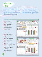
The Format dialog box appears
for the object you selected.
Here, it is the Format Chart
Title dialog box.
4
Click a tab.
5
Change the formatting
options.
6
Repeat Steps 4 and 5 to set
other formatting options.
7
Click Close.

Excel applies the formatting.
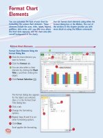
Format Chart Elements Using the
Format Dialog Box
1
Click the chart element you
want to format.
2
Click the Format tab.

•
You can also select a chart
element by clicking the Chart
Title
and then clicking the
object.
3
Click Format Selection ( ).
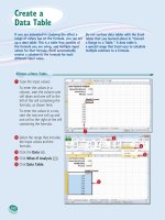
Format Chart Elements
You can customize the look of your chart by
formatting the various chart elements. These
elements include the axes, titles, labels, legend,
gridlines, data series, plot area (the area where
the chart data appears), and the chart area (the
overall background of the chart).
You can format chart elements using either the
Format dialog box or the Ribbon. The rest of
the sections in this chapter provide you with
more detail on using the Ribbon commands.
Format Chart
Elements
14_577639-ch12.indd 20014_577639-ch12.indd 200 3/15/10 2:48 PM3/15/10 2:48 PM
201
Formatting Excel Charts
CHAPTER
12
22
33
11
2

Click the Format tab.
3
Use the Ribbon controls to
change the formatting options.
Note: Not all of the Ribbon
controls will be available for each
chart element.

Excel applies the formatting.
Format Chart Elements Using the
Ribbon
1
Click the chart element you
want to format.
Are there any formatting shortcuts I can use?
Yes. Excel offers several methods you can use to
quickly open the Format dialog box. If you are
using your mouse, position
over the element
you want to format, and then double-click. From
the keyboard, first click the chart element you
want to format and then press
+ . You can
also right-click the chart element and then click
Format Element (where Element is the name of
the element).
How do I know where to click to
select a chart element?
The easiest way to be sure you are clicking
the correct element is to position

over
the object. If
is positioned correctly, a
banner appears and the banner text
displays the name of the chart element.
If the banner does not appear, or if the
banner displays a chart element name
other than the one you want to format,
move
until the correct banner appears.
14_577639-ch12.indd 20114_577639-ch12.indd 201 3/15/10 2:48 PM3/15/10 2:48 PM
202
22
11
33
44
•
Excel formats the element’s
background with the color you
selected.
Apply a Color Fill
1
Click the chart element you
want to format.
2
Click the Format tab.
3
Click the Shape Fill .
4
Click the color you want to

apply.
Customize a Chart Element Background
You can add visual interest to a chart element
by customizing the element’s background, or
what Excel calls the fill.
Most fills consist of a single color, but you can
also apply a color gradient, a texture, or even a
picture. However, you should be careful about
the background you choose for certain chart
elements. Since some chart elements —
particularly the chart area, plot area, value axis,
and category axis — display data, be sure to
choose a background that does not make that
data difficult to read.
Customize a Chart
Element Background
14_577639-ch12.indd 20214_577639-ch12.indd 202 3/15/10 2:48 PM3/15/10 2:48 PM
203
Formatting Excel Charts
CHAPTER
12
22
33
44
55
11
22
33
44
55

11
How do I use a picture as an element’s background?
Follow these steps:
1
Follow Steps 1 to 3.
2
Click Picture.
3
Click the folder that contains the image file.
4
Click the image file you want to use as the
background.
5
Click Insert.
Apply a Texture Fill
1
Click the chart element you
want to format.
2
Click the Format tab.
3
Click the Shape Fill .
4
Click Texture.
5
Click the texture you want to
apply.
•
Excel formats the element’s
background with the texture

you selected.
Apply a Gradient Fill
1
Click the chart element you
want to format.
2
Click the Format tab.
3
Click the Shape Fill .
4
Click Gradient.
5
Click the gradient you want to
apply.
•
Excel formats the element’s
background with the gradient
you selected.
33
44
55
14_577639-ch12.indd 20314_577639-ch12.indd 203 3/15/10 2:48 PM3/15/10 2:48 PM
204
22
33
11
55
66
77
44

5
Click the Shape Outline .
6
Click Weight.
7
Click the line thickness you
want to apply.
1
Click the chart element you
want to format.
2
Click the Format tab.
3
Click the Shape Outline .
4
Click the color you want
to apply.
Set a Chart Element’s Outline
You can make a chart element stand out by
customizing the element’s outline, which refers
to the border that appears around the element,
as well as to single-line elements, such as
gridlines and axes.
You can customize the outline’s color, its
weight — that is, its thickness — and whether
the line is solid or consists of a series of dots or
dashes.
Set a Chart
Element’s Outline
14_577639-ch12.indd 20414_577639-ch12.indd 204 3/15/10 2:48 PM3/15/10 2:48 PM