bài giảng thống kê thí nghiệm công nghệ thực phẩm phân tích số liệu bằng RPhân tích đồ thị
Bạn đang xem bản rút gọn của tài liệu. Xem và tải ngay bản đầy đủ của tài liệu tại đây (2.44 MB, 55 trang )
1
Tổng quan
Số liệu
Đồ thị cột- Barchart
Đồ thị tần số- Histogram
Đồ thị đường thẳng-Stripchart
Đồ thị hộp-Boxplot
Đồ thị xy- Scatter plot
Đồ thị Pie- Pie
2
Số liệu
Số liệu về thành phần của thân thể đo bằng
phương pháp hấp thu tia X
43 nam và nữ tuổi từ 11 đến 28
Tên biến:
id
age
sex
dur
weight
height
lm (lean mass)
pclm (percent lean mass)
fm (fat mass)
pcfm (percent fat mass)
bmc (bone mineral contents)
3
Đọc dữ liệu vào R
setwd(“D:/2016-XLSL”)
igfdata <- read.table(“igftxt.txt”, header=T)
attach(igfdata)
names(igfdata)
head(igfdata)
summary(igfdata)
……………………………………………..
Import data từ Rcmdr
[1] "id"
"age"
"sex"
"height" "lm"
"pclm"
[9] "fm"
"pcfm"
"dur"
"weight"
"bmc"
4
Distribution of gender
0
50
30
0
10
10
20
30
40
Frequency
50
60
Số lượng
Nữ
Nam
Giới tính
Female
Male
Gender
5
Xem số liệu
bc
id age sex
1
1 15
2
2 16
3
3 11
4
4 19
5
5 19
6
6 22
7
7 16
8
8 12
9
9 21
10 10 15
11 11 13
12 12 20
...
40 40 12
41 41 15
42 42 22
43 43 25
dur weight height
M
5
39
148
M
8
45
162
M
4
23
132
M
9
46
159
M
6
56
166
M 12
50
152
M
8
53
170
M
5
35
151
M
8
46
166
M
6
45
165
M
5
32
142
M
6
40
153
lm pclm
32.96 84.50
38.16 84.80
18.51 80.50
35.92 78.10
46.63 83.00
42.13 84.00
45.23 85.00
25.26 72.20
39.44 85.70
38.47 85.50
25.50 79.70
32.70 82.00
fm pcfm bmc
4.86 12.5 1.33
4.15 9.2 1.89
2.99 13.0 0.74
6.73 14.6 1.59
5.61 10.2 2.56
3.93 8.1 2.12
5.15 9.8 2.21
9.02 25.6 0.95
4.64 10.1 2.00
3.92 8.9 1.70
4.26 13.9 0.99
4.66 12.0 1.38
M
M
M
M
33.00
36.00
38.50
37.35
3.50 9.2 1.43
5.33 12.5 1.52
4.63 10.3 1.86
4.34 10.0 1.70
10
6
7
13
39
45
46
45
155
154
157
162
84.60
80.00
84.00
83.00
6
Tần số dạng cột: barplot
freq <- table(sex)
barplot(freq)
barplot(freq, horiz=T, main="Sex distribution")
0
5
F
10
15
20
M
25
30
Sex distribution
F
M
0
5
10
15
20
25
30
7
Distribution of gender
Frequency
40
30
Female
20
10
0
Frequency
50
Male
60
Distribution of gender
Female
Male
Gender
0
10
20
30
40
50
60
Gender
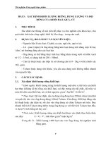
8
0
10
20
30
40
50
60
Tần số
Giới tính
Nữ
Nam
Hình 1.1. Biểu đồ phân bố giới tính
9
Tần số theo nhóm : barplot
0
5
10
15
20
25
agegroup <- cut(age, 3)
agesex <- table(sex, agegroup)
barplot(agesex)
(11,16.7]
(16.7,22.3]
(22.3,28]
10
Tần số theo nhóm : barplot
0
0
5
5
10
15
10
20
25
15
agegroup <- cut(age, 3)
agesex <- table(sex, agegroup)
barplot(agesex, xlab="Age group")
barplot(agesex, beside=T, xlab="Age group")
(11,16.7]
(16.7,22.3]
Age group
(22.3,28]
(11,16.7]
(16.7,22.3]
Age group
(22.3,28]
11
12
Female
Male
13
0
10
20
30
40
50
60
15
10
5
0
Tần số
20
25
Tần số nam và nữ
Nam
Nữ
Giới tính
Frequency of males and females
0
5
Nam
10
15
20
Nu
25
Frequency of males and females
Nam
Nu
0
10
15
20
25
Frequency of males and females
15
10
5
0
0
5
10
15
Tan so
20
20
25
25
Frequency of males and females
5
Nam
Nu
Nam
Nu
Gioi tinh
15
Phân phối số liệu: Histogram
Histogram of age
5
4
0
0
1
2
2
3
Frequency
6
4
Frequency
8
6
10
7
Histogram of age
15
20
25
15
20
age
Histogram of age
Histogram of age
25
6
5
4
3
2
1
0
0
1
2
3
4
Frequency
5
6
7
age
7
10
Frequency
par(mfrow=c(2,2))
hist(age)
hist(age, breaks=20)
hist(age, breaks=40)
hist(age, breaks=50)
15
20
age
25
15
20
age
25
16
Phân phối số liệu: Histogram
Histogram of weight
10
5
Frequency
6
4
0
0
2
Frequency
8
10
15
Histogram of age
15
20
25
20
30
40
50
age
weight
Histogram of lm
Histogram of fm
60
10
5
0
0
2
4
6
8
Frequency
15
10 12 14
10
Frequency
par(mfrow=c(2,2))
hist(age)
hist(weight)
hist(lm)
hist(fm)
15
20
25
30
35
lm
40
45
50
2
4
6
8
fm
10
12
14
17
Phân phối số liệu: Hàm mật độ-plot(density)
hist(age, main="Distribution of lean mass")
plot(density(age), main="Distribution of age")
Distribution of lean mass
0.02
0.03
Density
8
6
0.01
4
2
15
20
25
30
35
lm
40
45
50
0.00
0
Frequency
10
0.04
12
0.05
14
Distribution of lean mass
10
20
30
40
N = 43 Bandwidth = 2.607
50
18
Phân phối chuẩn? qqnorm
Normal Q-Q Plot
35
30
25
20
Sample Quantiles
40
45
qqnorm(lm)
-2
-1
0
Theoretical Quantiles
1
2
19
Tính liên tục của số liệu: stripchart
stripchart(age)
15
20
25
30
20
Boxplot
27
25
20
15
age
30
Boxplot(age~sex)
Female
Male
sex
21
Tính liên tục của số liệu: stripchart
stripchart(age, xlab=“Age; kg")
?
20
25
30
35
40
45
Lean mass; kg
22
Tóm tắt của số liệu liên tục:boxplot
boxplot(fm)
20
4
25
6
30
8
35
10
40
12
45
boxplot(lm)
LM
Min. 1st Qu.
18.51 31.91
Median
35.92
Mean 3rd Qu.
35.65
40.14
FM
Min. 1st Qu.
2.990 4.250
Median
5.270
Mean 3rd Qu.
Max.
6.500
8.795 12.800
Max.
46.63
23
Tóm tắt của số liệu liên tục: boxplot
Fat mass by sex
Lean mass by sex
boxplot(fm ~ sex)
20
4
25
6
30
8
35
10
40
12
45
boxplot(lm ~ sex)
F
M
F
M
24
Phân tích mức độ liên kết: scatter plot
plot(lm ~ age, pch=16)
lm
20
20
25
25
30
30
lm
35
35
40
40
45
45
plot(lm ~ age)
15
20
age
25
15
20
25
age
25